STATSEI14 · PRACTICAL TUTORIAL

Deep Learning
Meets ETAS

Practical Hybrid Workflows for Seismic Forecasting

Francisco Plaza-Vega
Universidad de Santiago de Chile

13 October 2026 · Chile

30 minutes of concepts and research · 30 minutes of guided practice

duration_seconds: 30

Main idea: Deep learning connects a representation to a scientific task.

Explain: We will spend 30 minutes on concepts and research, then 30 minutes on guided practice with LSTM, a Transformer comparison and closing discussion. ETAS supplies one way to construct a representation.

Transition: How do we turn catalogue history into a probability forecast, and what changes when we change the model?

Backup: Main slides s01–s20 end at minute 30. Return to d01 at minute 50 and h01 at minute 57.

What can we learn from seismicity?

Signals reveal recorded events.

Catalogues describe event histories.

Models turn histories into questions about what may follow.

What information do we represent, and what do we ask a model to learn?

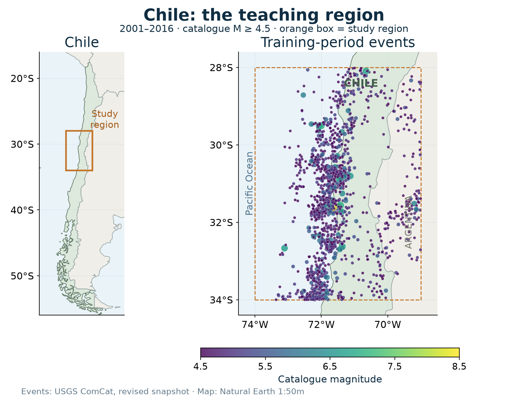
Map: frozen USGS training catalogue and Natural Earth. Illustrates today’s regional setting.

duration_seconds: 120

Main idea: The observation, representation and output determine the learning problem.

Explain: Signals record ground motion. A catalogue summarizes detected events. A model uses a chosen history to estimate a specified output. Learning adjusts weights from examples, but we choose the representation and target.

Transition: The next studies illustrate distinct choices of input and output. Our practical begins with a catalogue and ends with a weekly probability.

Backup: Map from today’s frozen USGS training benchmark with Natural Earth coastlines. It is not the CSN catalogue used in the published case. Observation is incomplete and catalogue records can change.

Deep learning in seismology: inputs and targets

Example	Input	Learning task
ConvNetQuake · 2018	Recorded waveforms	Detect events and classify their source region
RECAST · 2023	Past event times and magnitudes	Estimate the next-event time distribution
Delgado et al. · 2025	Features of catalogued events	Classify foreshock, mainshock and aftershock labels
Farfán et al. · 2025	Sequences of daily spatial grids	Forecast gridded seismic activity

Today’s practical: 30 days of history and a seven-day occurrence probability.

Perol et al. · Dascher-Cousineau et al. · Delgado et al. · Farfán et al.

duration_seconds: 210

Main idea: These applications answer different questions.

Explain each example:

• ConvNetQuake: a CNN detects events and classifies their source region from recorded waveforms. In our practical, those events are already represented in a catalogue.
• RECAST: a recurrent GRU summarizes past event times and magnitudes to model the next-event time distribution. Its benchmark is temporal ETAS. We will use daily inputs and a weekly occurrence target instead.
• Delgado et al.: event features support classification after spatial and temporal clustering and labeling. Labels such as foreshock, mainshock and aftershock show why target construction belongs to the scientific problem.
• Farfán et al.: sequences of daily 4 × 4 Chilean grids support forecasts of gridded activity. Spatial aggregation anticipates the maps and graphs available after our regional exercise.

Transition: We now introduce the network components needed to learn one of these mappings, then apply them to a common catalogue forecasting problem.

Backup: This selection is not a performance ranking. Event classification does not establish prospective warning. RECAST’s temporal benchmark does not establish superiority over spatial ETAS. Grid labels omit fine epicentre and magnitude information. Sources are linked on the slide. End the context block at minute 6.

A network learns a mapping from examples

Represented data → Neural network → Defined output

Compare with a target → Compute a loss → Update weights

Architecture determines how information is combined.

Training adjusts weights to reduce the loss.

The output and the loss must match the scientific question.

duration_seconds: 75

Main idea: Training changes weights to connect represented inputs with a defined output.

Explain: A history enters the network, an estimate comes out, and a loss measures its discrepancy from the target. Backpropagation computes gradients, and an optimizer updates the weights. Architecture determines how information is combined.

Transition: We will recognize this same loop in every network and in the notebook’s compile, fit and predict calls.

Backup: Validation guides choices and stopping. It does not update weights through backpropagation. Adapted from Units 1 and 2 of the author’s course.

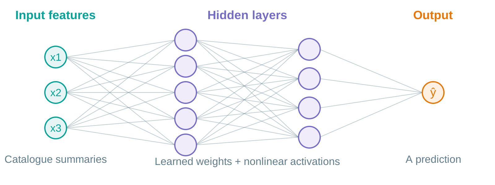
MLP: combine measured features

A multilayer perceptron learns nonlinear combinations of a feature vector.

Temporal laboratory: the MLP uses 90 values at fixed lag positions. Diagram adapted from the author’s DL course, Unit 2.

duration_seconds: 60

Main idea: An MLP combines a vector of measured features through learned layers.

Explain: Follow one connection and then one hidden layer. Weighted combinations and nonlinear activations compose a mapping. In the temporal laboratory section, flattening the 30 × 3 window gives 90 values, each at a fixed lag position.

Transition: The MLP is available for independent comparison. Next, shared filters use the local structure of a sequence.

Backup: Flattening preserves fixed lag positions. It does not randomly discard order. The guided session focuses on LSTM and Transformer. Diagram provenance: slides/assets/course-adapted/source-map.md.

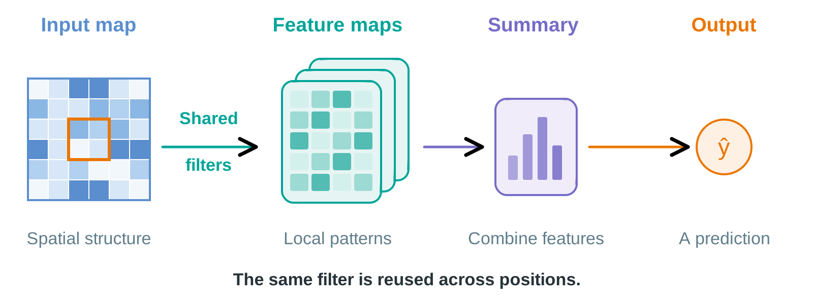
CNN: learn local patterns with shared filters

The same filter examines different neighborhoods.

Temporal laboratory: CNN1D shares filters across days. Diagram adapted from the author’s DL course, Unit 3.

duration_seconds: 75

Main idea: A convolution applies shared filters to local neighborhoods.

Explain: Use the diagram to identify a local receptive field and shared weights. In the temporal tutorial, CNN1D moves filters across days. In the published case, the CNN processes spatial patterns in ETAS-derived maps.

Transition: A recurrent model offers another way to combine the daily history by updating a state.

Backup: CNN1D is available after the live route as an optional laboratory section. The grid or temporal sampling determines what counts as a neighborhood. No kernel arithmetic is needed here. Diagram adapted from Unit 3 of the author’s course.

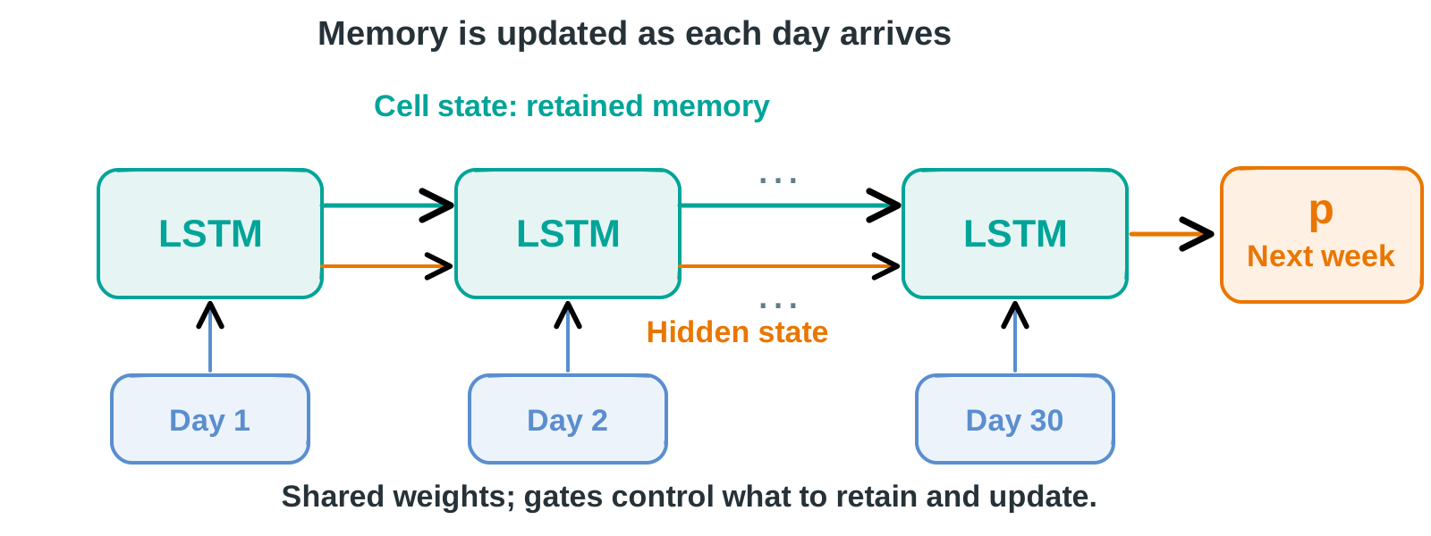
LSTM: carry information through a sequence

A learned state summarizes the history for a defined output.

Same learned update across time. Adapted from the author’s DL course, Unit 4.

duration_seconds: 90

Main idea: An LSTM summarizes a sequence through a learned state.

Explain: Read left to right. Each update combines the new day’s channels with information from previous days. Gates control what is retained, updated and exposed. A many-to-one model turns a 30-day input into one output.

Transition: This is the architecture we will explain in detail in Colab. A generative task asks for a richer output than one probability.

Backup: The published temporal case and today’s practical use different targets. Keep gate equations optional. At minute 50 we compare recurrence with attention on the same daily tensor.

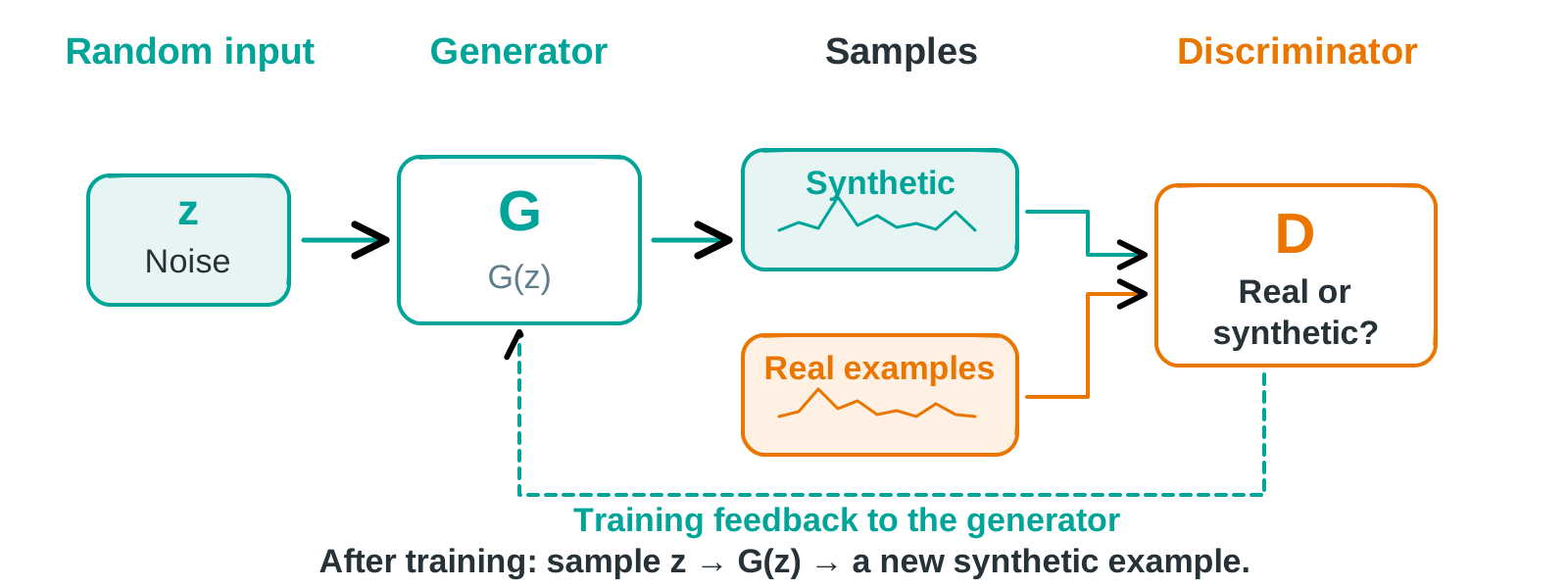
Generative learning: produce new samples

A generator learns to produce samples from a learned distribution.

GAN is one approach to generative learning. Adapted from the author’s DL course, Unit 5.

duration_seconds: 60

Main idea: A generator learns to produce samples under a training objective.

Explain: Random input allows different generated samples. A GAN uses a discriminator or critic to supply the generator’s training signal. The Isidora case also conditions generation on mainshock information.

Transition: With this vocabulary, consider how our first study turned an ETAS representation into neural inputs and targets.

Backup: Generative learning describes a task and can use MLP, CNN or recurrent components. A plausible curve alone does not establish a scientifically adequate distribution. End the concepts block at minute 12.

Our first case: learning from an ETAS representation

Scientific question

Can neural networks learn the evolution of a statistical representation of seismic activity?

Two views

A daily time series and a sequence of spatial maps.

Nicolis, Plaza & Salas · Spatial Statistics 42 (2021), 100442 · CSN Chile, 2000–2017

duration_seconds: 90

Main idea: The published study learns the evolution of an ETAS-derived representation.

Explain: Use the original author-provided workflow to identify the catalogue, representation and two neural branches. The daily time series and spatial maps create different inputs and outputs.

Transition: What does the ETAS representation measure before a neural network uses it?

Backup: Nicolis, Plaza & Salas, Spatial Statistics 42 (2021), 100442. Source: https://doi.org/10.1016/j.spasta.2020.100442 . Catalogue: CSN Chile, 2000–2017. Interpret the original intensity/location labels as model-derived targets, not physical shaking or an exact next epicentre.

ETAS supplies a statistical description of activity

\lambda(t\mid\mathcal H_t)=\mu+\sum_{t_i<t}\text{contribution from event }i

Background + magnitude-dependent contributions that decay with time

Spatial ETAS also describes how contributions vary over space.

This conditional occurrence rate becomes a representation for learning.

Conceptual sketch. Process intensity is different from magnitude and shaking intensity.

duration_seconds: 90

Main idea: ETAS describes a conditional event rate through background and past-event contributions.

Explain: Use the equation as a bridge from statistical seismology. Larger and more recent events can contribute differently. Spatial ETAS also models how contributions vary over space. The study summarizes the fitted intensity for learning.

Transition: A daily maximum creates a specific temporal prediction task.

Backup: Full estimation requires parameters, units and observation assumptions. Process intensity differs from magnitude, shaking intensity and probability. The appendix keeps those distinctions available.

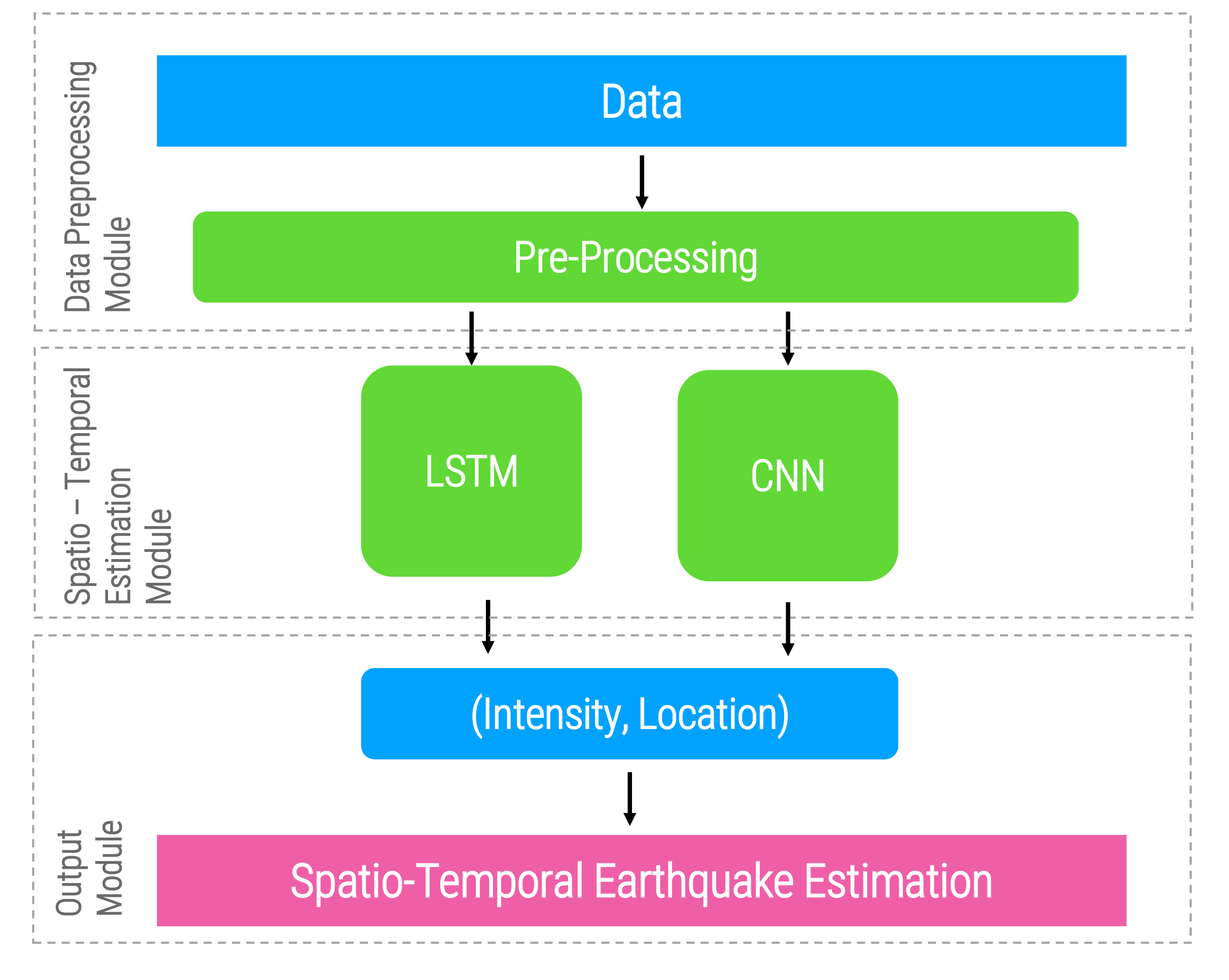
The temporal task: tomorrow’s maximum intensity

30 daily maxima → LSTM → Next-day maximum

Input and target: summaries of the ETAS-derived intensity.

Learning question: how much of its evolution can a temporal network capture?

Specify what is being predicted before interpreting a fit statistic.

Published case, Nicolis, Plaza & Salas (2021). The target is a model-derived quantity.

duration_seconds: 90

Main idea: This LSTM predicts a model-derived intensity summary.

Explain: Thirty daily maximum intensity values enter the network, and the next day’s maximum is the target. This example shows how a statistical representation makes a learning task possible.

Transition: Keeping a spatial map instead of one daily maximum opens a different output question.

Backup: The paper reports test R-squared of about 0.66 at the threshold-six setting. At threshold five, ETAS has lower MSE, MAE and RMSE. The paper does not establish that ETAS estimation excluded all test information. These qualifications prevent a claim of uniform neural superiority.

The spatial task: the macrozone of the maximum

30 daily ETAS maps → CNN → Six zone probabilities

Which macrozone contains tomorrow’s maximum estimated intensity?

The representation determines which information the network can use.

Published case, Nicolis, Plaza & Salas (2021). These probabilities concern six macrozones.

duration_seconds: 90

Main idea: Changing the representation changes which information the network can use.

Explain: Thirty daily ETAS maps feed the spatial branch. Its six probabilities concern the macrozone containing tomorrow’s maximum estimated intensity.

Transition: In that study ETAS supplied the representation. In our practical we construct simpler daily channels directly from the catalogue. In both settings, we must decide what the network receives and what its output means. With Isidora we explored a richer output: an aftershock sequence.

Backup: The macrozone is not the exact next epicentre or today’s fixed-box occurrence target. End the published-case block at minute 18.

With Isidora: can we generate aftershock sequences?

Mainshock conditions + noise → Generator → A possible sequence

Thesis question

Can conditional generative models reproduce the temporal pattern of aftershock sequences?

Model families explored

Conditional GAN · WGAN-GP · attention-based generator

A richer output requires us to decide what a sequence actually represents.

Isidora Jara Muñoz (2025), thesis · Subsequent manuscript by Plaza-Vega, Jara, Nicolis & Salinas (2026), under review

duration_seconds: 90

Main idea: Conditional generation asks for possible sequences following a mainshock.

Explain: Distinguish the mainshock conditions from the random input. The thesis explored conditional GAN, WGAN-GP and an attention-based generator. WGAN-GP changes the adversarial objective and regularization, while attention changes information exchange across positions.

Transition: Before judging the generated sequence, we must define what each entry represents.

Backup: Keep Isidora Jara Muñoz’s 2025 thesis separate from the 2026 manuscript by Plaza-Vega, Jara, Nicolis & Salinas, under review. TGAN in the thesis and GANT in the manuscript have separate evaluations. ETAS-GAN is outside the manuscript’s empirical scope.

One sequence mixes absence and magnitude

Representation in the manuscript

14 days → 224 intervals of 90 minutes → maximum magnitude per occupied interval

2.5 2.5 4.1 2.5 3.4 2.5 2.5 5.0

Schematic values. Gray: absence marker. Orange: maximum magnitude in an occupied interval.

“No recorded event” and “event magnitude” are different outcomes.

duration_seconds: 75

Main idea: This sequence representation combines absence with magnitude.

Explain: Fourteen days become 224 intervals of 90 minutes. The value 2.5 marks absence, while an occupied bin stores its maximum magnitude. Ask which information a maximum discards.

Transition: We therefore need to check event occupancy as well as numeric sequence errors.

Backup: The eight displayed values are schematic. Empty-bin 2.5 is not an observed magnitude. Occupied intervals are not the total number of aftershocks because a bin can contain multiple events.

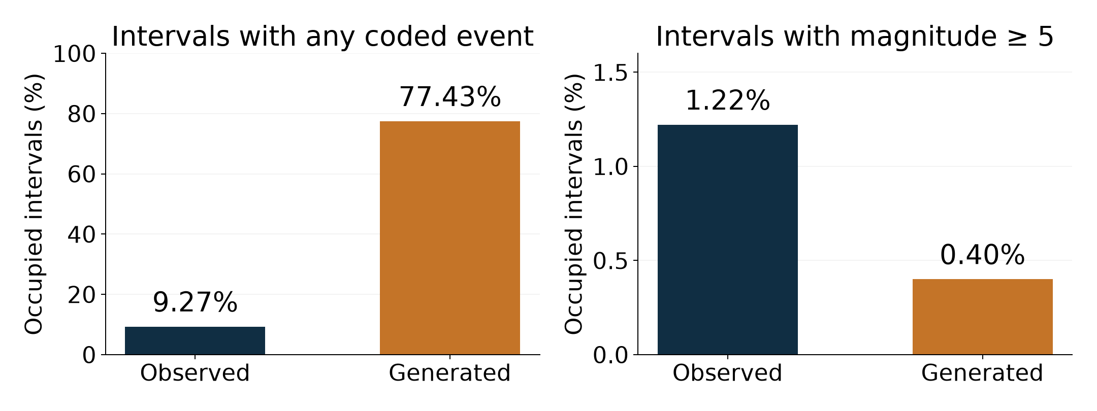
Generated sequences distort event occupancy

Assess which properties of the observed sequences are reproduced.

2026 manuscript under review · Occupied intervals, not total events · Source-case results

duration_seconds: 105

Main idea: Evaluation must test the properties the representation is intended to preserve.

Explain: The manuscript’s temporal evaluation shows too many occupied intervals overall and too few in the larger-magnitude subset. A curve-level fit measure cannot replace these checks.

Transition: These findings motivated closer attention to the target, including aggregate occurrence and exceedance outcomes.

Backup: Source: Table_gant_temporal_blocked_event_occupancy.csv. Overall occupancy is 9.27% observed and 77.43% generated. Reported M≥5 occupancy is 1.22% and 0.40%, but inherited threshold code has > versus ≥ ambiguity. Temporal GANT mean-baseline skill is −13.8%. Original PI uses a mean reference, not last-observation persistence. Keep thesis, illustrative and blocked results separate. These findings do not establish failure of all generative models.

The article revisits what the model should learn

Empirical reformulation

Aggregate targets: occurrence, exceedance and count summaries.

The classification branch uses tree models.

A future neural formulation

Occurrence probability, followed by magnitude conditional on occurrence.

Evaluate both parts and their joint behavior.

Today we isolate occurrence in a fixed future interval as the learning target.

ETAS-informed generation remains future work. The two-part neural model is a proposal.

duration_seconds: 90

Main idea: The target deserves as much scrutiny as the architecture.

Explain: The revised manuscript examines aggregate occurrence, exceedance and count targets with Random Forest and Gradient Boosting. Separating occurrence probability from conditional magnitude is a future neural proposal.

Transition: This experience led us to examine the target more carefully. Today’s exercise isolates occurrence within a fixed future interval, giving us a clear output to train and evaluate before considering richer sequence models.

Backup: Do not attribute tree-model classification scores to GANs or LSTMs. Ranking performance varies with temporal and geographic evaluation and does not imply calibrated operational warning. Some inherited horizons were not fully purged. The proposed two-part neural model is unvalidated. End the research cases at minute 24.

The practical puts the same decisions in your hands

Case	Representation	Output
Spatial Statistics	ETAS time series and maps	Intensity maximum and its macrozone
Isidora / manuscript	Mainshock conditions; binned sequences	Conditional sequences; aggregate targets
Today	Daily catalogue channels	Weekly occurrence probability

Live: LSTM and Transformer. Laboratory extensions: MLP, CNN1D, maps and graphs.

duration_seconds: 75

Main idea: The same modeling decisions connect the research cases and our exercise.

Explain: Spatial Statistics contributes the representation question. The Isidora work contributes the target question. Today we build a regional weekly probability from daily catalogue channels.

Transition: The live route uses the linear temporal notebook: build one example, define references, train the LSTM, evaluate its probabilities and compare with a Transformer. MLP, CNN1D, maps, graphs and the earlier activity score remain extensions.

Backup: Today’s task does not reproduce either study. Building the notebook from a blank Colab is an independent-study route. Keep the prepared results available if setup or training stalls.

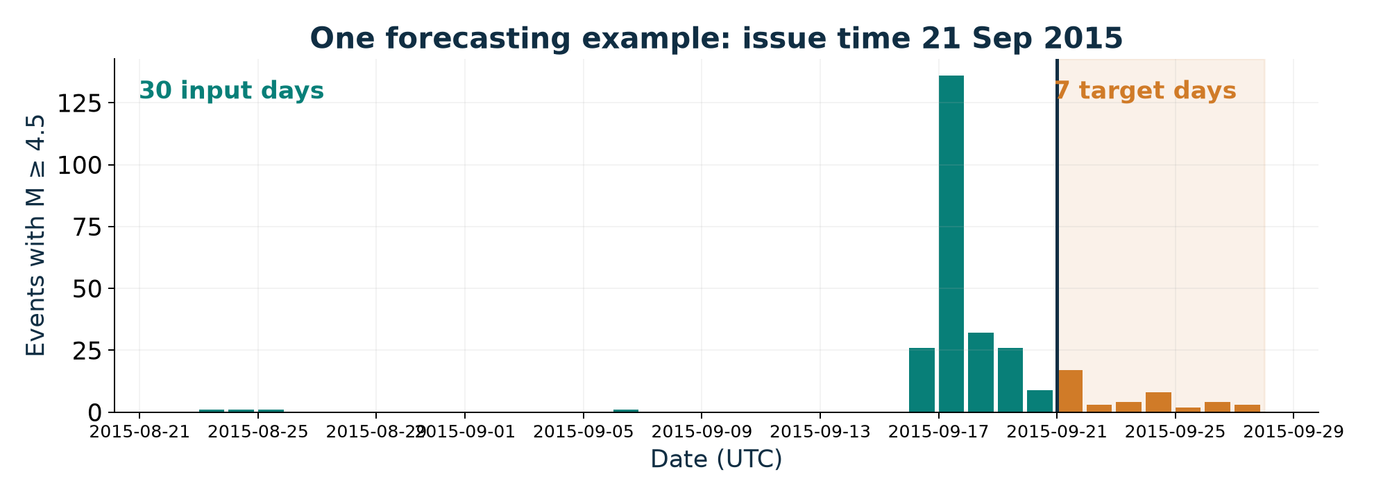
Today’s target: at least one event next week

30 past days → probability of at least one catalogue M ≥ 5 event in seven days.

One input: 30 days × 3 channels · Region: 28–34°S, 69–74°W · Input M ≥ 4.5 · Monday origins

duration_seconds: 105

Main idea: One example is a 30-day input window and the label for its following week.

Explain: Point to the history, Monday forecast origin and seven-day target before showing code. The input has shape 30 × 3: log event count, maximum magnitude excess above 4.5, and an event indicator. The label is one if at least one catalogue M≥5 event occurs in the region during that week.

Transition: How should these examples be divided for learning and evaluation?

Backup: An empty day and an event exactly at M=4.5 both have zero excess, but different event indicators. Inputs are examples × days × channels. ComCat mixes magnitude scales. The thresholds are teaching choices, not proof of completeness. The target does not specify exact location, shaking or damage.

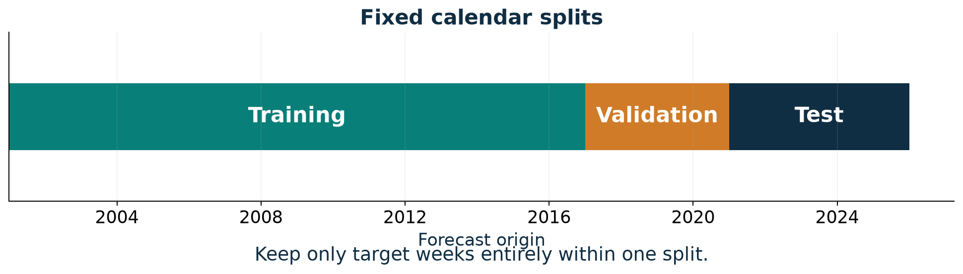
Evaluate using the temporal order of the problem

Today we compare validation probabilities using Brier score, log loss and calibration.

Train 2001–2016 · Validation 2017–2020 · Test 2021–2025 was inspected previously and is excluded from this comparison.

duration_seconds: 90

Main idea: The current temporal tutorial compares validation performance only.

Explain: Training determines weights and normalization. Validation controls early stopping and supplies today’s probability diagnostics. The older test interval was already inspected during course development and is excluded from the current comparison. Target weeks cannot cross a partition boundary.

Transition: Compare the LSTM with training prevalence and logistic regression, then process the same history with a Transformer.

Backup: Training 2001–2016, validation 2017–2020, historical test 2021–2025. Earlier experiments retain their own test results. The revised frozen ComCat catalogue does not reconstruct historical availability. Validation used for stopping is development evidence. A sigmoid does not guarantee calibration.

Experiment: how does the same history enter each model?

30 days × 3 catalogue channels → LSTM → weekly probability

The same history → Transformer → the same target

Build one example: identify the input window, its origin and its label.

Train and evaluate: read compile, fit, predict and compare probability errors.

What changes when different architectures process the same information?

Prepared temporal notebook · Seed 7 · MLP and CNN1D for the laboratory · Activity-score experiment as an extension

duration_seconds: 90

Main idea: The exercise changes the architecture while retaining the daily history and occurrence target.

Explain: First identify an example and fit simple references. Then read the LSTM definition followed immediately by compile, fit, predict and its probability scores. The Transformer reuses the same 30 × 3 tensor and evaluation.

Transition: Open the prepared temporal notebook at minute 30.

Backup: Minutes 30–34: setup and one window. Minutes 34–43: references and LSTM. Minutes 43–50: scores, calibration and interpretation. Minutes 50–57: Transformer using d01–d03. Minutes 57–60: discussion using h01. At minute 34, use prepared outputs if setup is incomplete. Use prepared outputs if a fit exceeds three minutes. The activity-score exercise belongs to the earlier practical and remains an optional extension. Main slides sum to 1,800 seconds.

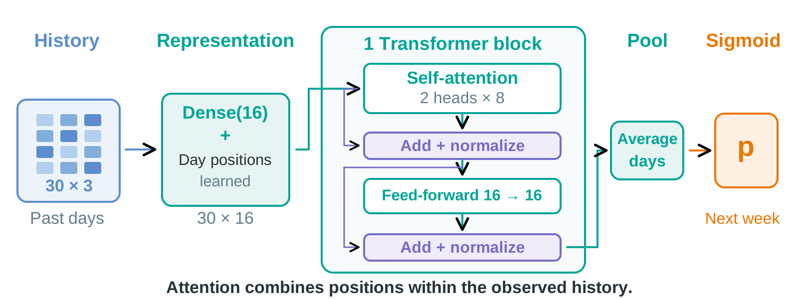
A Transformer combines the same history differently

Same history and target. A different way to combine information across days.

Current temporal tutorial · 2,257 trainable parameters versus 1,297 for LSTM · One fixed, small configuration

duration_seconds: 120

Main idea: Attention combines the same observed days differently from an LSTM state.

Explain: At minute 50, show the current temporal notebook’s Transformer. Each day is projected to 16 features and receives a learned 16-value day-position embedding. Two attention heads, each with key dimension 8, combine positions. Residual additions and layer normalization surround attention and the 16-to-16 feed-forward sublayer. Average pooling and a sigmoid produce the weekly probability.

Transition: At minute 52, compare the probabilities under the unchanged evaluation.

Backup: The diagram matches the explicit Transformer definition in scripts/linear_tutorial_sources/temporal.json. Projection: 64 parameters, learned positions: 480, attention: 1,088, two normalizations: 64, feed-forward: 544, output: 17. Total: 2,257 trainable parameters versus 1,297 for LSTM. No dropout is applied. All input positions precede the origin, so within-history attention does not expose the target. Capacity differs between architectures. Attention weights alone do not establish causation.

Validation probabilities from one declared seed

Model	Validation Brier	Validation log loss
Training prevalence	0.187690	0.562855
Logistic regression	0.203664	0.614405
LSTM	0.181521	0.547512
Transformer	0.187901	0.562477

Lower is better. Compare these scores with the calibration plot and its sample counts.

These are development results from one region and one validation period.

Linear temporal tutorial · One fit per neural model, seed 7 · 208 validation origins · Logistic regression uses all 90 lagged values

duration_seconds: 180

Main idea: A probability score summarizes the errors of one fitted model on the validation weeks.

Explain: Use minutes 52–55 to inspect the model summary, prepared predictions and calibration. The displayed neural scores each come from one fit with seed 7. Training prevalence and logistic regression each have one result. Logistic regression receives all 90 lagged channel values. Both neural models receive the same 30 × 3 input. In this seed-7 run, the LSTM has lower Brier and log loss than the Transformer and both references. The Transformer and constant reference have similar losses. Compare both scores without assuming that added complexity improves them.

Transition: Which conclusions do these scores support, and which require a new experiment?

Backup: Source: results/linear/temporal/validation_metrics.csv. There are 208 validation origins. A single seed does not measure sensitivity to initialization. The separate repeated temporal comparison retains seeds 7, 17 and 27 and reports its own means. Validation also selects stopping, so it is not independent assessment. The earlier Transformer pilot used fixed sinusoidal positions and summary-feature logistic regression, and its scores are separate evidence. Do not mix that pilot’s test table or the repeated comparison’s means with this table. Use prepared results if live fitting stalls.

What can this result tell us about the problem?

Reading the validation results

Compare each model with training prevalence.

Read Brier, log loss and calibration together.

Questions for the next experiment

Which representation and target preserve useful structure?

What information is available in the catalogue?

Would more data, capacity or a different training budget change the result?

Useful deep learning depends on how we represent the phenomenon and formulate the task.

Validation also controls early stopping. One seed does not measure initialization sensitivity.

duration_seconds: 120

Main idea: A score difference does not explain its cause.

Explain: Use minutes 55–57 to connect the comparison to our cases. Spatial Statistics supplied a fitted representation. The Isidora work exposed difficulties in the output definition. Here, each model has one declared fit on the same history. An observed score difference describes those settings; it does not explain why the models differ.

Transition: Ask for one testable hypothesis and the comparison needed to investigate it, then choose an extension for the laboratory.

Backup: This comparison cannot isolate representation, information availability, sample size, optimization or capacity as a cause. It does not establish that attention is unsuitable for seismicity. Validation is development evidence, and the historical test was already inspected. New claims need a documented protocol and appropriate fresh evaluation.

What did we learn, and what would we test next?

1. What information did our daily channels preserve or discard?
2. What did the LSTM and Transformer comparison establish?
3. Which extension would you test next: maps, graphs or an activity score?

Deep learning offers flexible tools. Their scientific value depends on the question and the evidence.

Homework: guided reading or a controlled extension · Build on today’s LSTM and Transformer comparison

duration_seconds: 180

Main idea: Scientific usefulness depends on the question and the evidence supporting the model.

Explain: Close at minutes 57–60. Invite two brief interpretations of the fixed-input architecture comparison. Distinguish the observed loss from a proposed explanation. Ask what spatial information was lost when the catalogue was pooled over the region.

Transition: Choose a continuation: maps, graphs, another temporal model or the earlier activity-score extension. The homework guide sets out reading and controlled experiments for the laboratory.

Backup: Keep baselines, a stated hypothesis and the evaluation protocol. The earlier feature experiment is a different comparison from today’s architecture exercise. Participants with less Python experience can use prepared outputs and guided reading. Thirty minutes of presentation plus thirty minutes of practical work, including comparison and discussion, total sixty minutes.

Appendix · the LSTM steps

inputs = keras.Input(shape=(30, 3))
state = keras.layers.LSTM(16)(inputs)
probability = keras.layers.Dense(1, activation="sigmoid")(state)
model_lstm = keras.Model(inputs, probability)
model_lstm.compile(optimizer="adam", loss="binary_crossentropy")
history_lstm = model_lstm.fit(
    X_train, y_train, validation_data=(X_val, y_val),
    epochs=20, batch_size=64, callbacks=[stopping_lstm], shuffle=False)
p_lstm = model_lstm.predict(X_val).ravel()
brier = np.mean((p_lstm - y_val) ** 2)

Define the model · compile · fit · predict · evaluate probabilities

Abbreviated reference for the linear practical. The notebook sets seed 7 and prepares training-only scaling. Beside compile, it defines stopping_lstm with patience 3 and restored best weights. The notebook specifies Adam learning rate 0.001 explicitly. Validation selects stopping rather than updating weights through gradients. Each operation appears next to the model it concerns. https://keras.io/api/layers/recurrent_layers/lstm/ .

Appendix · quantities and scientific meaning

Quantity	Question answered
Process intensity	At what conditional rate do events occur?
Magnitude	How large is an event?
Shaking intensity	What motion or effects occur at a location?
Risk	What consequences may occur given exposure and vulnerability?

Today’s output is a probability of a defined occurrence event.

The published title and original workflow labels require this distinction. ETAS intensity is an event rate. A probability for an interval needs a predictive calculation, not relabeling a rate. None of today’s probability scores is a shaking or damage estimate.

Appendix · earlier activity-score extension

r_t(s)=\sum_{t-L\le t_i<s}10^{\alpha(M_i-M_0)} \left(1+\frac{s-t_i}{c}\right)^{-p},\quad s\le t.

Illustrative: α=1, c=1 day, p=1.1, L=30 days.

Earlier feature experiment: both LSTMs use the same available history.

Representation: log1p(score) is an additional daily channel.

Optional extension from the earlier practical. The illustrative index is not a fitted ETAS rate.

Earlier optional feature experiment. These results are separate from the current temporal architecture comparison. The history is truncated separately at each origin and the daily endpoint includes only strictly earlier events. A fitted ETAS extension needs a documented estimation sample, units, observation model and forecast construction. For the optional 14-day task, both variants use L=14. The binary target is at least one catalogue event M>=5 in [t,t+7 days).

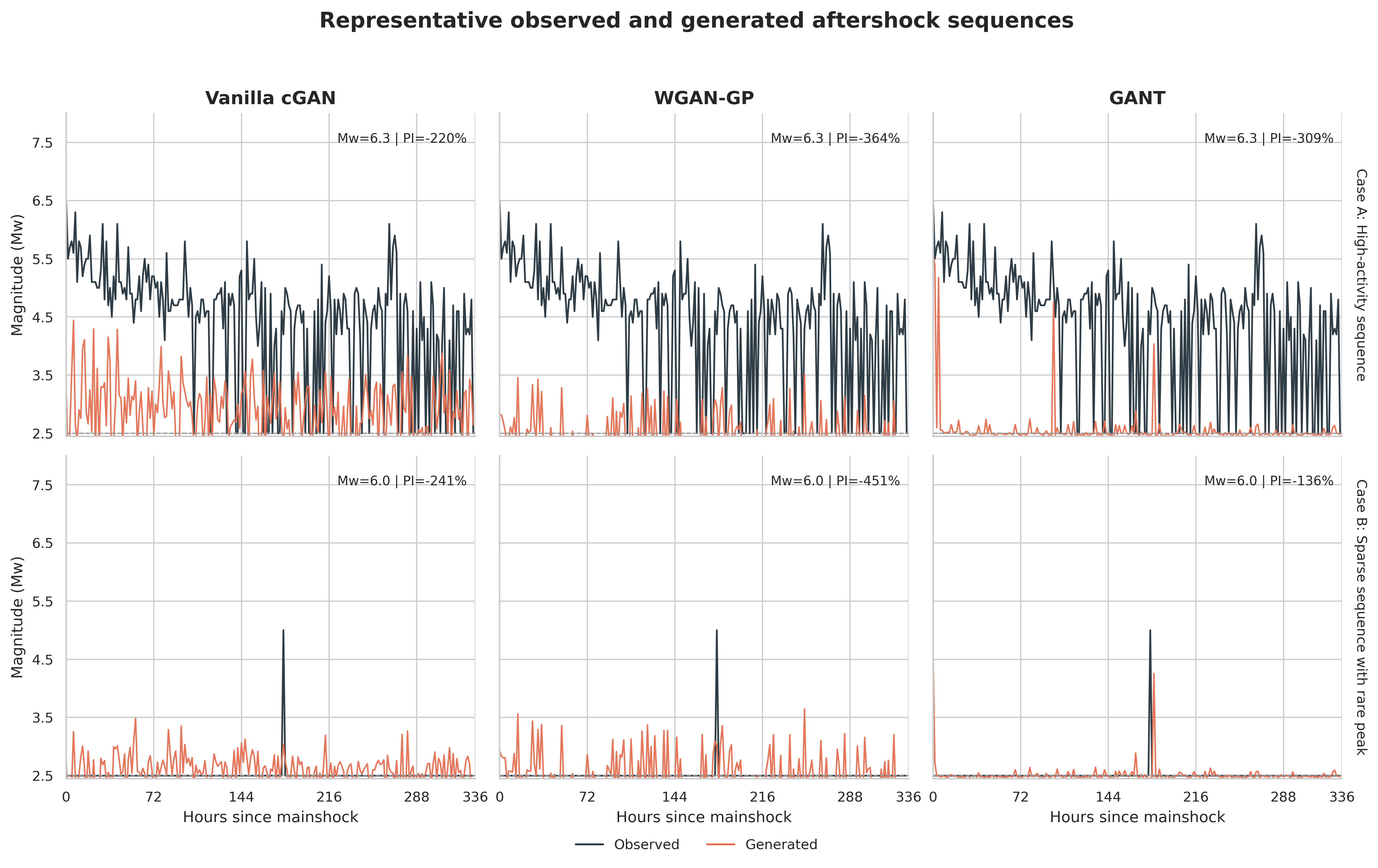
Appendix · original generative examples

2026 manuscript under review · Original PI annotations use a mean-reference denominator · Illustrative cases

Use only if discussion requires the original sequence examples. These panels are not the blocked-evaluation occupancy comparison. The absence marker is 2.5; occupied-bin maxima discard multiplicity. Original PI is a mean-baseline measure rather than last-observation persistence. Do not merge illustrative case values with the aggregate temporal evaluation or thesis results.

Appendix · evidence and availability

Check	Meaning
Chronological, purged targets	Future target intervals do not cross partitions.
Training-only normalization	Later inputs do not set scaling parameters.
Frozen revised catalogue	Data bytes and provenance are reproducible.
Historical catalogue vintages	Not reconstructed.

Reproducibility and historical information availability are separate requirements.

Magnitude, location and inclusion may have changed after an event. The updated field is not first publication and cannot reconstruct original versions or label-adjudication delays. Dependent weeks, one regional split and a small number of seeds limit generalization. The linear temporal tutorial reports validation only, with seed 7 once per neural model. The separate repeated comparison retains seeds 7, 17 and 27. The earlier activity-score run uses one seed and the earlier Transformer pilot uses three. Those earlier experiments retain their own test results, which are not a fresh evaluation for the current tutorial. A source or architecture’s reported score should not be transferred to a different target.

Appendix · sources and further reading

• Seismic applications: ConvNetQuake · RECAST.
• Our published case: Nicolis, Plaza & Salas (2021).
• Generative case: Jara Muñoz (2025), thesis; Plaza-Vega, Jara, Nicolis & Salinas (2026), manuscript under review.
• Attention context and further reading: Delgado et al. (2025) · Farfán et al. (2025).
• Diagram style: author’s DL course, Units 2–5 · Transformer schematic matches the current temporal tutorial.
• Materials: practical · homework · full references.

Context papers are distinct tasks, not a ranking of architectures. The 2026 manuscript status is under review, confirmed by the author. Original course diagram sources and any inherited attribution are preserved in slides/assets/course-adapted/source-map.md. Full private theses and manuscripts are excluded from distribution. Foundational DL and data/software references remain on the references page.