One history, four neural architectures — Three-seed reference comparison
Live: understand an LSTM, evaluate probabilities, then compare a Transformer
Download prepared notebook Open Colab to upload the notebook Notebook with prepared outputs Blank Colab for self-study All tutorials
This page retains the original repeated experiment (seeds 7, 17 and 27), its code and prepared outputs. Its averages and spreads belong to that experiment. For the 30-minute practical and direct single-seed code, use the linear teaching walkthrough. Do not substitute these outputs for an execution of the linear notebook.
How do we turn catalogue history into a probability forecast, and what changes when we change the model? This tutorial follows the 30-minute presentation with a 30-minute practical. Open the notebook with cells already prepared, execute in order, and focus the live discussion on the LSTM, probability evaluation, and the Transformer. The full executable comparison also includes an MLP and a CNN1D for follow-up study.
First, understand one observation
Imagine that today is a Monday, the forecast origin t. Before making the forecast, we look at the 30 complete days before t. For each day we record three numbers:
| Daily channel | Meaning and example |
|---|---|
log_count |
Before standardization: log(1 + count) of catalogue events with M >= 4.5. Two events give log(3). |
max_magnitude_excess |
Before standardization: maximum magnitude excess above 4.5; zero if there is no event. A daily maximum of 5.2 gives 0.7. |
has_event |
Before standardization: 1 if at least one M >= 4.5 event occurred, otherwise 0. Two events give 1. |
These numbers form one input window of shape 30 x 3: 30 days, three channels. They are a conceptual example, not an extra observed result. The label is 1 if at least one M >= 5 event occurs in the next seven days, from this Monday through the following Sunday, and 0 otherwise. That future week is excluded from the input. A sigmoid output such as 0.30 is a probability for this binary outcome, not a predicted magnitude or an exact earthquake date.
Checkpoint before any code: point to the input history, the forecast origin, and the target week. One observation is a weekly forecast window, not one earthquake.
The live 30-minute route
Times below are minutes from the beginning of the full 60-minute session; the presentation occupies 00-30.
| Session minutes | Live discussion | Where to look |
|---|---|---|
| 30-34 | Open the prepared notebook; identify one 30 x 3 window and its label; begin sequential execution | This example and the shared preparation |
| 34-43 | Compare the two references; read the LSTM definition and the training call | Sections 2, 5, and 7 |
| 43-50 | Interpret LSTM probabilities, Brier score, log loss, and calibration | Sections 8-9; use the prepared outputs if the run is still busy |
| 50-57 | Compare how the Transformer uses the same history and inspect its results | Return to section 6, then revisit sections 8-9 |
| 57-60 | State one finding, one limitation, and one next experiment | Section 10 and After class |
Run code in order; choose what to explain in depth. The short MLP, CNN1D, and Transformer definition cells must execute before the common training cell. That cell retains all four architectures and all three seeds. During the live explanation, concentrate on the LSTM first and return to the Transformer afterwards; detailed MLP/CNN1D discussion belongs to the complete study route. No fresh training is needed to read the supplied local outputs.
Open the prepared notebook in Colab
For the live practical, download the notebook with cells already prepared. Open Google Colab, choose File > Upload notebook, and select temporal.ipynb. Select a Python CPU runtime and run the cells from the beginning in order. Keep this page alongside Colab for the explanations. The separate notebook with prepared outputs is a reference from the documented local run.
Execution order and teaching order serve different purposes. Run all code cells in sequence so every variable and model definition exists. The instructor will pause the explanation at selected checkpoints while execution continues. If setup or training takes longer than the live slot, read the prepared local outputs on this page; completing a fresh run can continue after class. Do not skip code cells just because their detailed explanation is deferred.
For self-study from a blank notebook: open a new Colab and copy each numbered Python block into its own code cell, in order. The Copy button copies code only. This produces the same experiment as the prepared notebook.
The first run downloads a frozen public data pack automatically. Its URL is pinned to a Git commit and its SHA-256 is checked. There is no manual ZIP upload and no live catalogue query. After an interrupted session, run the notebook again from the beginning. Outputs below labelled prepared local run come from an independent local CPU execution; they are not a claim about your Colab session.
Colab normally supplies the required libraries. If imports fail, install tensorflow==2.19.1 pandas scikit-learn matplotlib in a separate cell with %pip install, restart the runtime, and begin again. Exact local versions and timings are recorded with the prepared results. Installation changes the active Colab environment only.
Prepare the environment
We use small networks and three predeclared seeds. A seed controls the pseudo-random choices used for initialization and optimization; it does not represent uncertainty from new earthquakes. The tutorials evaluate validation only: the existing course test period has already been inspected. Changing architecture now does not make that period an untouched test again.
Code block 1 · Run the matching prepared-notebook cell in order. For self-study, copy into a new Colab code cell.
import os
os.environ["CUDA_VISIBLE_DEVICES"] = "-1"
os.environ["TF_CPP_MIN_LOG_LEVEL"] = "2"
os.environ["TF_NUM_INTRAOP_THREADS"] = "2"
os.environ["TF_NUM_INTEROP_THREADS"] = "2"

from pathlib import Path
import datetime, hashlib, json, platform, time, uuid, zipfile
from urllib.request import urlopen
import numpy as np
import pandas as pd
import matplotlib.pyplot as plt
import sklearn
import tensorflow as tf
from tensorflow import keras
from IPython.display import display

try:
    tf.config.threading.set_intra_op_parallelism_threads(2)
    tf.config.threading.set_inter_op_parallelism_threads(2)
except RuntimeError:
    print("Thread settings were already initialized; restart for the reference settings.")

SEEDS = [7, 17, 27]
EPOCHS, BATCH_SIZE = 20, 64
TUTORIAL = "temporal"
RUN_DIR = Path("tutorial-runs") / (TUTORIAL + "-" + uuid.uuid4().hex[:12])
RUN_DIR.mkdir(parents=True, exist_ok=False)
started_at = time.perf_counter()
print("Python:", platform.python_version(), "TensorFlow:", tf.__version__, "Keras:", keras.__version__)
print("Validation only. Results will be saved to", RUN_DIR)
Prepared local output — expand to compare
Python: 3.12.14 TensorFlow: 2.19.1 Keras: 3.15.1
Validation only. Results will be saved to tutorial-runs\temporal-0da80b1f5731
Download and verify the frozen catalogue
The pack contains the regional USGS catalogue and its provenance. It includes records down to M 3 for diagnostics; these tutorials retain M ≥ 4.5 as inputs and M ≥ 5 as targets. Magnitudes are the preferred catalogue values, not a claim that all measurements use the same magnitude scale.
The catalogue was downloaded in October 2026 and contains revised records. Separating inputs and targets by event time cannot reconstruct which catalogue versions were available historically. These are retrospective teaching experiments, not operational forecasts or maps of shaking or risk.
Code block 2 · Run the matching prepared-notebook cell in order. For self-study, copy into a new Colab code cell.
PACK_URL = "https://raw.githubusercontent.com/FranPlaza/FranPlaza.github.io/0e7a7e4b1c38490018f11b26170fe6a87e4997f9/courses/statsei14/downloads/data-pack.zip"
PACK_SHA256 = "0ee5d4d71aafa19023fdb1ee6f289a11e7fd7f4ed88ad7a91032ca24505d10a2"
CATALOGUE_SHA256 = "16e9b731a5b407d75a2321d3d0d2c889542e8223a9ee4fe81efe624eb6b166d2"
archive_path = Path("statsei14-data-pack.zip")
if not archive_path.exists():
    with urlopen(PACK_URL, timeout=60) as response:
        payload = response.read()
    assert hashlib.sha256(payload).hexdigest() == PACK_SHA256, "Unexpected download: stop."
    archive_path.write_bytes(payload)
assert hashlib.sha256(archive_path.read_bytes()).hexdigest() == PACK_SHA256, "Changed cached pack: stop."
DATA_DIR = Path("statsei14-data").resolve()
DATA_DIR.mkdir(exist_ok=True)
with zipfile.ZipFile(archive_path) as archive:
    for member in archive.infolist():
        assert (DATA_DIR / member.filename).resolve().is_relative_to(DATA_DIR), "Unsafe ZIP member."
    archive.extractall(DATA_DIR)
catalogue_path = DATA_DIR / "data/frozen/usgs_chile_2000_2025.csv"
assert hashlib.sha256(catalogue_path.read_bytes()).hexdigest() == CATALOGUE_SHA256
events = pd.read_csv(catalogue_path)
events["time"] = pd.to_datetime(events["time"], utc=True)
events = events.sort_values("time").reset_index(drop=True)
print("Verified catalogue records:", len(events))
display(events[["time", "latitude", "longitude", "mag"]].head())
Prepared local output — expand to compare
Verified catalogue records: 12859
| time | latitude | longitude | mag | |
|---|---|---|---|---|
| 0 | 2000-01-07 11:49:11.720000+00:00 | -28.495 | -69.196 | 4.0 |
| 1 | 2000-01-08 11:43:58.150000+00:00 | -31.017 | -71.339 | 4.4 |
| 2 | 2000-01-11 13:16:34.420000+00:00 | -30.747 | -71.319 | 4.5 |
| 3 | 2000-01-18 17:12:18.360000+00:00 | -31.630 | -71.451 | 4.9 |
| 4 | 2000-01-19 01:24:00.150000+00:00 | -31.440 | -71.384 | 3.8 |
Turn events into daily inputs
Each day has three channels: log(1 + count), maximum magnitude excess above 4.5 (the daily maximum minus 4.5, or zero on an empty day), and an event-presence indicator. The regional series pools all locations. For the spatial tutorials we also keep six fixed geographic cells: three latitude bands by two longitude bands. Cell IDs run west to east within each row, then south to north. They are illustrative geographic bins, not inferred tectonic provinces; degree-based cells do not have identical physical areas. We retain the same domain and magnitude thresholds for every model.
Only training data should be used to judge whether the grid has adequate support. A finer map would create more rare targets, not automatically more useful information. In Tutorial 1, X_regional is the input; the spatial arrays are prepared here so the three tutorials share one transparent data pipeline.
Code block 3 · Run the matching prepared-notebook cell in order. For self-study, copy into a new Colab code cell.
START = pd.Timestamp("2000-01-01", tz="UTC")
END = pd.Timestamp("2026-01-01", tz="UTC")  # exclusive
days = pd.date_range(START, END - pd.Timedelta(days=1), freq="D")
LAT_EDGES = np.array([-34.0, -32.0, -30.0, -28.0])
LON_EDGES = np.array([-74.0, -71.5, -69.0])
N_ROWS, N_COLS = 3, 2
FEATURES = ["log_count", "max_magnitude_excess", "has_event"]
inside = events.latitude.between(LAT_EDGES[0], LAT_EDGES[-1]) & events.longitude.between(LON_EDGES[0], LON_EDGES[-1])
selected = events.loc[inside & (events.time >= START) & (events.time < END) & (events.mag >= 4.5)].copy()
selected["day"] = (selected.time.dt.floor("D") - START).dt.days
selected["row"] = np.clip(np.searchsorted(LAT_EDGES, selected.latitude, side="right") - 1, 0, N_ROWS - 1)
selected["col"] = np.clip(np.searchsorted(LON_EDGES, selected.longitude, side="right") - 1, 0, N_COLS - 1)

counts = np.zeros((len(days), N_ROWS, N_COLS), dtype=np.float32)
max_excess = np.zeros_like(counts)
target_counts = np.zeros_like(counts)
indices = (selected.day.to_numpy(), selected.row.to_numpy(), selected.col.to_numpy())
np.add.at(counts, indices, 1)
np.maximum.at(max_excess, indices, selected.mag.to_numpy() - 4.5)
qualifying = selected.mag.to_numpy() >= 5.0
np.add.at(target_counts, tuple(axis[qualifying] for axis in indices), 1)
daily_grid_raw = np.stack([np.log1p(counts), max_excess, (counts > 0).astype(float)], axis=-1).astype("float32")
daily_regional_raw = np.stack([
    np.log1p(counts.sum(axis=(1, 2))),
    max_excess.max(axis=(1, 2)),
    (counts.sum(axis=(1, 2)) > 0).astype(float)
], axis=-1).astype("float32")
assert int(counts.sum()) == len(selected)
assert int(target_counts.sum()) == int(qualifying.sum())
print("Daily regional:", daily_regional_raw.shape, "; daily grid:", daily_grid_raw.shape)
Prepared local output — expand to compare
Daily regional: (9497, 3) ; daily grid: (9497, 3, 2, 3)
Build histories, labels and chronological partitions
At each Monday origin t, inputs use [t − 30 days, t) and targets use [t, t + 7 days). We remove any target interval that crosses a train/validation/test boundary or the end of the catalogue. Inputs to a later partition can contain earlier historical days; their outcomes never enter training. Weekly target windows do not overlap, although histories overlap and earthquake sequences remain dependent.
The regional target is one binary outcome. The spatial target has six binary outcomes: several cells may be positive in the same week, or all may be zero. Six cell probabilities therefore need not sum to one.
Code block 4 · Run the matching prepared-notebook cell in order. For self-study, copy into a new Colab code cell.
LOOKBACK, HORIZON = 30, 7
VAL_START = pd.Timestamp("2017-01-01", tz="UTC")
TEST_START = pd.Timestamp("2021-01-01", tz="UTC")
regional_windows, grid_windows, grid_labels, kept_origins, partitions = [], [], [], [], []
excluded = []
for origin in pd.date_range("2001-01-01", "2025-12-31", freq="W-MON", tz="UTC"):
    i = (origin - START).days
    stop = origin + pd.Timedelta(days=HORIZON)
    split = "train" if origin < VAL_START else ("validation" if origin < TEST_START else "test")
    boundary = VAL_START if split == "train" else (TEST_START if split == "validation" else END)
    if i < LOOKBACK or stop > boundary:
        excluded.append(str(origin.date()))
        continue
    regional_windows.append(daily_regional_raw[i - LOOKBACK:i])
    grid_windows.append(daily_grid_raw[i - LOOKBACK:i])
    grid_labels.append((target_counts[i:i + HORIZON].sum(axis=0) > 0).astype("int32"))
    kept_origins.append(origin)
    partitions.append(split)
origins = pd.DatetimeIndex(kept_origins)
partitions = np.asarray(partitions)
raw_regional = np.stack(regional_windows)
raw_grid = np.stack(grid_windows)
y_grid = np.stack(grid_labels)
y_regional = y_grid.any(axis=(1, 2)).astype("int32")
train_mask = partitions == "train"
val_mask = partitions == "validation"
test_mask = partitions == "test"
assert np.all(origins[train_mask] + pd.Timedelta(days=HORIZON) <= VAL_START)
assert np.all(origins[val_mask] + pd.Timedelta(days=HORIZON) <= TEST_START)
assert np.all(origins[test_mask] + pd.Timedelta(days=HORIZON) <= END)
assert not np.any(train_mask & val_mask)
print("Windows:", dict(zip(*np.unique(partitions, return_counts=True))))
print("Excluded boundary/incomplete targets:", excluded)
display(pd.DataFrame({
    "cell": np.arange(N_ROWS * N_COLS),
    "row_south_to_north": np.repeat(np.arange(N_ROWS), N_COLS),
    "col_west_to_east": np.tile(np.arange(N_COLS), N_ROWS),
    "training_positive_weeks": y_grid[train_mask].sum(axis=0).reshape(-1),
    "training_base_rate": y_grid[train_mask].mean(axis=0).reshape(-1)
}))
Prepared local output — expand to compare
Windows: {np.str_('test'): np.int64(260), np.str_('train'): np.int64(834), np.str_('validation'): np.int64(208)}
Excluded boundary/incomplete targets: ['2016-12-26', '2020-12-28', '2025-12-29']
| cell | row_south_to_north | col_west_to_east | training_positive_weeks | training_base_rate | |
|---|---|---|---|---|---|
| 0 | 0 | 0 | 0 | 57 | 0.068345 |
| 1 | 1 | 0 | 1 | 26 | 0.031175 |
| 2 | 2 | 1 | 0 | 49 | 0.058753 |
| 3 | 3 | 1 | 1 | 37 | 0.044365 |
| 4 | 4 | 2 | 0 | 19 | 0.022782 |
| 5 | 5 | 2 | 1 | 41 | 0.049161 |
Standardize using training histories only
For regional inputs, we estimate one mean and standard deviation per channel. For spatial inputs, we also use one pair per channel, pooled across training cells, so the map and graph models receive exactly the same scaled arrays. Empty days remain distinguishable through the presence channel. Target labels are never standardized.
The metric function averages squared probability errors and binary log losses. On spatial outputs these are averages of marginal cell scores, not the likelihood of a joint spatial point process. We will also inspect each cell separately.
Code block 5 · Run the matching prepared-notebook cell in order. For self-study, copy into a new Colab code cell.
regional_mean = raw_regional[train_mask].mean(axis=(0, 1), dtype=np.float64)
regional_scale = raw_regional[train_mask].std(axis=(0, 1), dtype=np.float64)
regional_scale = np.where(regional_scale > 0, regional_scale, 1.0)
grid_mean = raw_grid[train_mask].mean(axis=(0, 1, 2, 3), dtype=np.float64)
grid_scale = raw_grid[train_mask].std(axis=(0, 1, 2, 3), dtype=np.float64)
grid_scale = np.where(grid_scale > 0, grid_scale, 1.0)
X_regional = ((raw_regional - regional_mean) / regional_scale).astype("float32")
X_grid = ((raw_grid - grid_mean) / grid_scale).astype("float32")
assert X_regional.shape[1:] == (30, 3) and X_grid.shape[1:] == (30, 3, 2, 3)
assert np.isfinite(X_regional).all() and np.isfinite(X_grid).all()

def score_probabilities(y_true, probability):
    y_true = np.asarray(y_true, dtype=float)
    probability = np.asarray(probability, dtype=float)
    assert y_true.shape == probability.shape
    assert np.isin(y_true, [0, 1]).all() and np.isfinite(probability).all()
    assert ((probability >= 0) & (probability <= 1)).all()
    clipped = np.clip(probability, 1e-7, 1 - 1e-7)
    return {"brier": float(np.mean((probability - y_true) ** 2)),
            "log_loss": float(-np.mean(y_true * np.log(clipped) + (1 - y_true) * np.log1p(-clipped)))}

protocol = {
    "tutorial": TUTORIAL, "seeds": SEEDS, "epochs_max": EPOCHS, "batch_size": BATCH_SIZE,
    "lookback_days": LOOKBACK, "horizon_days": HORIZON,
    "pack_url": PACK_URL, "pack_sha256": PACK_SHA256, "catalogue_sha256": CATALOGUE_SHA256,
    "features": FEATURES, "latitude_edges": LAT_EDGES.tolist(), "longitude_edges": LON_EDGES.tolist(),
    "train": "2001-2016", "validation": "2017-2020", "test": "2021-2025; not evaluated here",
    "historical_as_of_verified": False, "scope": "Exploratory retrospective; validation only",
    "regional_mean": regional_mean.tolist(), "regional_scale": regional_scale.tolist(),
    "grid_mean": grid_mean.tolist(), "grid_scale": grid_scale.tolist(),
    "python": platform.python_version(), "tensorflow": tf.__version__, "keras": keras.__version__,
    "numpy": np.__version__, "pandas": pd.__version__, "scikit_learn": sklearn.__version__
}
(RUN_DIR / "protocol.json").write_text(json.dumps(protocol, indent=2), encoding="utf-8")
pd.DataFrame({"origin": origins.astype(str), "split": partitions}).to_csv(RUN_DIR / "windows.csv", index=False)
print("Ready:", X_regional.shape, X_grid.shape, "; no test outcomes used for fitting or evaluation.")
Prepared local output — expand to compare
Ready: (1302, 30, 3) (1302, 30, 3, 2, 3) ; no test outcomes used for fitting or evaluation.
1. One question, four ways to read a sequence
The target is the probability of at least one catalogue event with M ≥ 5 in the next seven days anywhere in the course region. Every model receives the same preceding 30 days and the same three catalogue channels: log event count, maximum magnitude excess above 4.5, and an event indicator. The shared preparation above standardizes the channels using training windows only.
An MLP uses fixed lag positions; a CNN1D shares filters across time; an LSTM updates a recurrent state; a Transformer relates days through attention and position information. Flattening for the MLP keeps each lag in a fixed position: it does not randomly discard order.
We retain the existing chronological split: training 2001–2016, validation 2017–2020, and historical test 2021–2025. Since the historical test has already informed earlier course development, this extension compares validation performance only. Validation also controls early stopping, so these scores are development evidence, not an independent estimate of future performance. The revised catalogue does not establish what records were available in real time.
Checkpoint. A row represents one weekly forecast origin, not one earthquake. Why should we avoid a random split of these rows?
Live checkpoint (30-34). Match the arrays below to the conceptual window: (number of windows, 30, 3) contains many histories, while each target is a single 0 or 1. For the next step, keep the same inputs and target while changing only how a model reads them.
Code block 6 · Run the matching prepared-notebook cell in order. For self-study, copy into a new Colab code cell.
from sklearn.linear_model import LogisticRegression

FEATURE_NAMES = ['log_count', 'max_magnitude_excess', 'has_event']
assert X_regional.ndim == 3 and X_regional.shape[1:] == (30, 3)
assert len(y_regional) == len(X_regional) == len(origins)
assert np.isfinite(X_regional).all()
assert set(np.unique(y_regional)).issubset({0, 1})
assert not np.any(train_mask & val_mask)
assert not np.any((train_mask | val_mask) & test_mask)

X_train = X_regional[train_mask].astype('float32')
X_val = X_regional[val_mask].astype('float32')
y_train = y_regional[train_mask].astype('float32')
y_val = y_regional[val_mask].astype('float32')
assert len(np.unique(y_train)) == len(np.unique(y_val)) == 2
assert pd.DatetimeIndex(origins[train_mask]).max() < pd.DatetimeIndex(origins[val_mask]).min()

partition_table = pd.DataFrame([
    {'split': 'training', 'windows': len(y_train), 'positive_fraction': y_train.mean()},
    {'split': 'validation', 'windows': len(y_val), 'positive_fraction': y_val.mean()},
])
display(partition_table)
print('Training input:', X_train.shape, '| Validation input:', X_val.shape)
print('Features:', FEATURE_NAMES)
print('Historical test is not evaluated in this tutorial.')
Prepared local output — expand to compare
| split | windows | positive_fraction | |
|---|---|---|---|
| 0 | training | 834 | 0.236211 |
| 1 | validation | 208 | 0.250000 |
Training input: (834, 30, 3) | Validation input: (208, 30, 3)
Features: ['log_count', 'max_magnitude_excess', 'has_event']
Historical test is not evaluated in this tutorial.
2. Start with two reference forecasts
The prevalence forecast assigns every validation week the training positive fraction. Logistic regression receives the same 90 values as the MLP, with fixed L2 regularization. Neither reference is tuned on validation. A neural network must be compared with these inexpensive alternatives before its extra complexity is interpreted as useful.
Brier score measures squared probability error; log loss penalizes confident wrong predictions strongly. Smaller values are better for both. We record runtime, but a single Colab session is not a hardware benchmark.
Live checkpoint (34-43). The training prevalence asks what happens if we give every week the same probability. Logistic regression uses all 30 x 3 = 90 lagged values with 91 fitted coefficients including the intercept. Neither is the older course logistic model built from a smaller feature summary. Compare the LSTM against these current references.
If a week has outcome 1, predicting 0.8 contributes (0.8 - 1)^2 = 0.04 to Brier score; predicting 0.2 contributes 0.64. The score averages these errors across weeks. Log loss is especially sensitive to being confident and wrong. Calibration asks a different question: among weeks assigned similar probabilities, how often does the event occur?
Code block 7 · Run the matching prepared-notebook cell in order. For self-study, copy into a new Colab code cell.
metric_rows = []
prediction_frames = []
training_histories = {}
validation_predictions = {}
validation_origins = pd.DatetimeIndex(origins[val_mask])

def record_run(name, seed, probabilities, parameters, epochs, seconds):
    p = np.asarray(probabilities, dtype=float).reshape(-1)
    assert p.shape == y_val.shape and np.isfinite(p).all()
    assert np.all((p >= 0) & (p <= 1))
    metric_rows.append({
        'model': name, 'seed': seed,
        **score_probabilities(y_val, p),
        'parameters': int(parameters), 'epochs': int(epochs),
        'fit_seconds': float(seconds),
    })
    validation_predictions[(name, seed)] = p
    prediction_frames.append(pd.DataFrame({
        'origin': validation_origins, 'model': name, 'seed': seed,
        'observed': y_val.astype(int), 'probability': p,
    }))

training_prevalence = float(y_train.mean())
record_run('Training prevalence', None, np.full(len(y_val), training_prevalence), 1, 0, 0)

started = time.perf_counter()
logistic = LogisticRegression(C=1.0, solver='lbfgs', max_iter=2000)
logistic.fit(X_train.reshape(len(X_train), -1), y_train)
logistic_seconds = time.perf_counter() - started
assert logistic.n_iter_.max() < logistic.max_iter, 'Inspect logistic convergence before comparing.'
p_logistic = logistic.predict_proba(X_val.reshape(len(X_val), -1))[:, 1]
record_run('Logistic regression', None, p_logistic,
           logistic.coef_.size + logistic.intercept_.size, 0, logistic_seconds)
display(pd.DataFrame(metric_rows))
Prepared local output — expand to compare
| model | seed | brier | log_loss | parameters | epochs | fit_seconds | |
|---|---|---|---|---|---|---|---|
| 0 | Training prevalence | None | 0.187690 | 0.562855 | 1 | 0 | 0.000000 |
| 1 | Logistic regression | None | 0.203664 | 0.614405 | 91 | 0 | 0.016523 |
3. MLP: learn from fixed lag positions (complete study route)
Flatten changes (30, 3) into (90,) without changing the order of the values. A dense hidden layer can combine channels and days, but does not share the same pattern detector across lag positions.
Checkpoint. Where would the value for the most recent day appear after flattening? What changes if the same temporal pattern shifts five days earlier?
Execute this definition in order. The common training cell needs build_mlp; the live route does not need a line-by-line explanation here.
Code block 8 · Run the matching prepared-notebook cell in order. For self-study, copy into a new Colab code cell.
def build_mlp(input_shape):
    inputs = keras.Input(shape=input_shape, name='history')
    x = keras.layers.Flatten(name='fixed_lag_positions')(inputs)
    x = keras.layers.Dense(16, activation='relu', name='hidden')(x)
    outputs = keras.layers.Dense(1, activation='sigmoid', name='weekly_probability')(x)
    return keras.Model(inputs, outputs, name='MLP')
4. CNN1D: look for local temporal patterns (complete study route)
A kernel of width 3 examines three adjacent days at a time, across all input channels. The next convolution combines nearby responses. Global average pooling summarizes the detected patterns before the probability output. This deliberately compact example favors patterns that can appear at different lag positions; it does not preserve every exact lag in the final pooled vector.
The convolution slides over days, not geographic locations. See the Keras time-series CNN example for another application of this idea.
Checkpoint. What useful information might shared filters capture? What exact timing information might pooling lose?
Execute this definition in order. The common training cell needs build_cnn1d; return for the detailed comparison after the live session.
Code block 9 · Run the matching prepared-notebook cell in order. For self-study, copy into a new Colab code cell.
def build_cnn1d(input_shape):
    inputs = keras.Input(shape=input_shape, name='history')
    x = keras.layers.Conv1D(16, kernel_size=3, padding='same', activation='relu',
                            name='local_patterns')(inputs)
    x = keras.layers.Conv1D(16, kernel_size=3, padding='same', activation='relu',
                            name='combined_patterns')(x)
    x = keras.layers.GlobalAveragePooling1D(name='pool_days')(x)
    outputs = keras.layers.Dense(1, activation='sigmoid', name='weekly_probability')(x)
    return keras.Model(inputs, outputs, name='CNN1D')
5. LSTM: update a state through the history
The LSTM processes the sequence from the oldest day to the most recent day. Its gates determine how its learned state changes as each day is read. The final state feeds the same sigmoid probability output.
This is a stateless model: the state restarts for every 30-day window. We do not carry a hidden state between training and validation examples.
Checkpoint. Why is the final hidden state a representation of the input history rather than a forecast probability by itself?
Read the definition aloud (34-43). keras.Input describes one 30 x 3 history. LSTM(16) learns a 16-number summary while reading the days in order. Dense(1, activation='sigmoid') turns that summary into one probability between 0 and 1. keras.Model connects the input to the output; defining the model does not train it.
In the training cell, compile specifies how errors are measured and how weights are updated. model.fit then repeatedly presents training windows and their known labels to adjust those weights. An epoch is one pass through the training examples; a batch is the group of examples used for one update. Validation observations monitor the fit, and early stopping retains the epoch with the lowest validation log loss. These validation scores therefore remain development results.
Code block 10 · Run the matching prepared-notebook cell in order. For self-study, copy into a new Colab code cell.
def build_lstm(input_shape):
    inputs = keras.Input(shape=input_shape, name='history')
    x = keras.layers.LSTM(16, stateful=False, name='read_history')(inputs)
    outputs = keras.layers.Dense(1, activation='sigmoid', name='weekly_probability')(x)
    return keras.Model(inputs, outputs, name='LSTM')
6. Transformer: relate days using attention and positions
Each day is projected into 16 features. A small learned positional embedding tells the network which lag each row represents. Two attention heads combine information across the complete observed history; residual connections, normalization, and a feed-forward block refine that representation.
The position layer below exposes its weights explicitly through the public Keras layer API. It needs no custom installation or hidden helper. The Keras time-series Transformer example provides the broader architecture pattern; this teaching adaptation adds explicit day positions and uses the course’s fixed chronological splits.
A causal attention mask is unnecessary here: all 30 input days precede the forecast origin, and the model produces one probability for the subsequent week. No target-week observation is an input. Attention weights, if inspected later, would not establish physical causation.
Checkpoint. Without position information, which aspect of the sequence would attention followed by average pooling struggle to distinguish?
Live comparison (50-57). This model has 2,257 trainable parameters, including learned positions. Return to this definition after interpreting the LSTM. Both models receive exactly the same 30 x 3 history and produce the same kind of weekly probability; what changes is how they combine information across days. Compare their current validation rows against the same two references, then inspect calibration. More flexible interactions do not guarantee better probabilities.
Code block 11 · Run the matching prepared-notebook cell in order. For self-study, copy into a new Colab code cell.
@keras.utils.register_keras_serializable(package='STATSEI14')
class DayPosition(keras.layers.Layer):
    def build(self, input_shape):
        self.positions = self.add_weight(
            name='positions',
            shape=(int(input_shape[1]), int(input_shape[2])),
            initializer=keras.initializers.RandomNormal(stddev=0.02),
            trainable=True,
        )
        super().build(input_shape)

    def call(self, inputs):
        return inputs + self.positions

    def get_config(self):
        return super().get_config()


def build_transformer(input_shape):
    inputs = keras.Input(shape=input_shape, name='history')
    x = keras.layers.Dense(16, name='project_day')(inputs)
    x = DayPosition(name='day_positions')(x)
    attention = keras.layers.MultiHeadAttention(
        num_heads=2, key_dim=8, dropout=0.0, name='attention')(x, x)
    x = keras.layers.Add(name='attention_residual')([x, attention])
    x = keras.layers.LayerNormalization(epsilon=1e-6, name='attention_norm')(x)
    feed_forward = keras.layers.Dense(16, activation='relu', name='ff_hidden')(x)
    feed_forward = keras.layers.Dense(16, name='ff_output')(feed_forward)
    x = keras.layers.Add(name='ff_residual')([x, feed_forward])
    x = keras.layers.LayerNormalization(epsilon=1e-6, name='ff_norm')(x)
    x = keras.layers.GlobalAveragePooling1D(name='pool_days')(x)
    outputs = keras.layers.Dense(1, activation='sigmoid', name='weekly_probability')(x)
    return keras.Model(inputs, outputs, name='Transformer')
7. Train with a common, small budget
Each architecture uses the same examples, batch size, optimizer, learning rate, maximum epochs, and stopping rule. The parameter counts differ and are reported; this is a controlled teaching comparison, not equal-compute tuning of every model family. EarlyStopping is recreated for every fit, monitors validation log loss, and restores the best weights.
Run once, in sequence. This cell fits all four models for each of the three seeds: 12 fits in total. Keep the preceding MLP, CNN1D, LSTM, and Transformer definitions even when the live explanation concentrates on the LSTM. Runtime depends on the session, and progress appears after each fit. The 30-minute teaching route is not a guarantee that a new Colab execution will finish within that time; the prepared local outputs keep each checkpoint available while a run continues.
Live checkpoint (34-43). Find model.fit(X_train, y_train, ...): training inputs and labels determine the weight updates; validation_data supplies the held-out development period used by early stopping. After fitting, model(X_val, training=False) produces probabilities without updating weights. Read the LSTM row first, then return to the Transformer during minutes 50-57. Keep all configured seeds for the recorded comparison. Seed variation reflects initialization and optimization, not uncertainty from observing a different earthquake catalogue.
The three channels stay unchanged across architectures. Adding an ETAS-inspired channel would be a separate input experiment.
Code block 12 · Run the matching prepared-notebook cell in order. For self-study, copy into a new Colab code cell.
BUILDERS = {
    'MLP': build_mlp,
    'CNN1D': build_cnn1d,
    'LSTM': build_lstm,
    'Transformer': build_transformer,
}
INPUT_SHAPE = tuple(X_train.shape[1:])
assert len(SEEDS) == len(set(SEEDS)) and len(SEEDS) >= 1

# Reset only this cell's previous neural runs if it is executed again.
metric_rows = [row for row in metric_rows if row['model'] not in BUILDERS]
prediction_frames = [frame for frame in prediction_frames
                     if frame['model'].iloc[0] not in BUILDERS]
validation_predictions = {key: value for key, value in validation_predictions.items()
                          if key[0] not in BUILDERS}
training_histories = {}

for name, builder in BUILDERS.items():
    for seed in SEEDS:
        keras.backend.clear_session()
        keras.utils.set_random_seed(seed)
        model = builder(INPUT_SHAPE)
        model.compile(
            optimizer=keras.optimizers.Adam(learning_rate=0.001),
            loss=keras.losses.BinaryCrossentropy(),
        )
        stopping = keras.callbacks.EarlyStopping(
            monitor='val_loss', patience=3, restore_best_weights=True,
        )
        started = time.perf_counter()
        history = model.fit(
            X_train, y_train,
            validation_data=(X_val, y_val),
            epochs=EPOCHS, batch_size=BATCH_SIZE,
            callbacks=[stopping], shuffle=False, verbose=0,
        )
        seconds = time.perf_counter() - started
        # All validation windows fit in memory; inference has no dropout or updates.
        p = model(X_val, training=False).numpy().reshape(-1)
        record_run(name, seed, p, model.count_params(),
                   len(history.history['loss']), seconds)
        training_histories[f'{name}_seed_{seed}'] = {
            key: [float(value) for value in values]
            for key, values in history.history.items()
        }
        scores = metric_rows[-1]
        print(f"{name:12s} seed={seed:2d} | params={model.count_params():4d} | "
              f"epochs={scores['epochs']:2d} | Brier={scores['brier']:.4f} | "
              f"log loss={scores['log_loss']:.4f} | {seconds:.1f}s")
Prepared local output — expand to compare
WARNING:tensorflow:From C:\Users\Francisco Plaza\AppData\Local\Temp\statsei14-transformer-pilot-20261007\Lib\site-packages\keras\src\backend\common\global_state.py:82: The name tf.reset_default_graph is deprecated. Please use tf.compat.v1.reset_default_graph instead.
MLP seed= 7 | params=1473 | epochs=20 | Brier=0.1918 | log loss=0.5789 | 1.4s
MLP seed=17 | params=1473 | epochs=16 | Brier=0.1982 | log loss=0.5897 | 1.1s
MLP seed=27 | params=1473 | epochs=20 | Brier=0.1956 | log loss=0.5946 | 1.3s
CNN1D seed= 7 | params= 961 | epochs=10 | Brier=0.1871 | log loss=0.5612 | 1.0s
CNN1D seed=17 | params= 961 | epochs=12 | Brier=0.1872 | log loss=0.5615 | 1.1s
CNN1D seed=27 | params= 961 | epochs=13 | Brier=0.1867 | log loss=0.5603 | 1.1s
LSTM seed= 7 | params=1297 | epochs=20 | Brier=0.1815 | log loss=0.5475 | 2.2s
LSTM seed=17 | params=1297 | epochs=20 | Brier=0.1836 | log loss=0.5518 | 2.2s
LSTM seed=27 | params=1297 | epochs=20 | Brier=0.1841 | log loss=0.5529 | 2.2s
Transformer seed= 7 | params=2257 | epochs= 6 | Brier=0.1879 | log loss=0.5625 | 1.6s
Transformer seed=17 | params=2257 | epochs= 5 | Brier=0.1901 | log loss=0.5674 | 1.5s
Transformer seed=27 | params=2257 | epochs= 5 | Brier=0.1883 | log loss=0.5635 | 1.5s
8. Read the full comparison
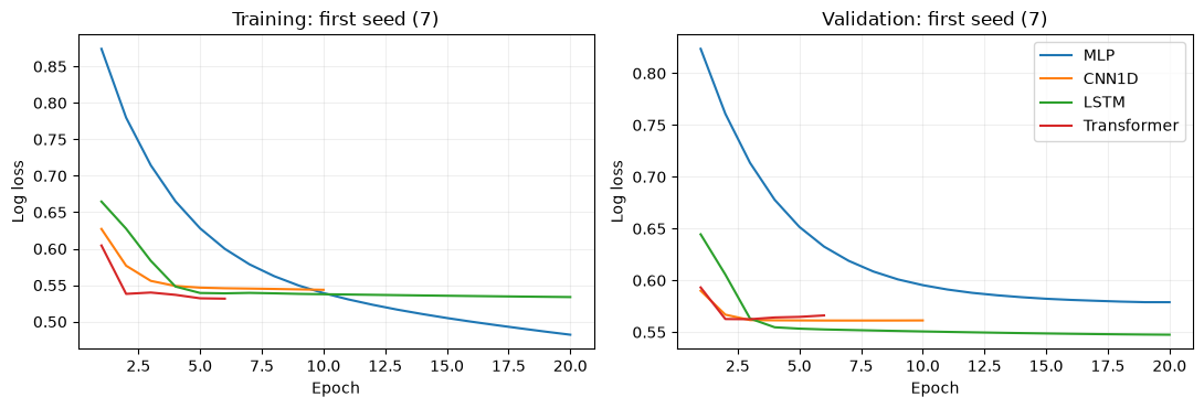
The first table retains every run. The second reports descriptive means and standard deviations across seeds; the deterministic baselines have one run, so their seed standard deviations are undefined. We display models in a fixed teaching order rather than choosing a winning seed.
Checkpoint. Does any architecture improve both probability scores over both references? Is the difference larger than the observed variation across seeds? A difference among these small implementations does not establish a universal ranking of MLPs, CNNs, LSTMs, and Transformers.
Live checkpoint (43-50). First read training prevalence, logistic regression, and LSTM. State whether the LSTM improves both scores and how its differences compare with seed variation. At minutes 50-57, add the Transformer row to the same comparison. The MLP/CNN1D rows remain visible for the complete study route. Do not compare this table with scores from the older ETAS-indicator experiment: the input representation and validation comparison are different.
Code block 13 · Run the matching prepared-notebook cell in order. For self-study, copy into a new Colab code cell.
model_order = ['Training prevalence', 'Logistic regression', *BUILDERS.keys()]
metrics = pd.DataFrame(metric_rows)
metrics['model'] = pd.Categorical(metrics['model'], categories=model_order, ordered=True)
metrics = metrics.sort_values(['model', 'seed']).reset_index(drop=True)
display(metrics.round(5))

summary = metrics.groupby('model', observed=True).agg(
    runs=('brier', 'size'),
    brier_mean=('brier', 'mean'), brier_seed_sd=('brier', 'std'),
    log_loss_mean=('log_loss', 'mean'), log_loss_seed_sd=('log_loss', 'std'),
    parameters=('parameters', 'first'),
    epochs_mean=('epochs', 'mean'), fit_seconds_mean=('fit_seconds', 'mean'),
).reindex(model_order)
display(summary.round(5))

fig, axes = plt.subplots(1, 2, figsize=(11, 3.8))
for name in BUILDERS:
    history = training_histories[f'{name}_seed_{SEEDS[0]}']
    epochs = np.arange(1, len(history['loss']) + 1)
    axes[0].plot(epochs, history['loss'], label=name)
    axes[1].plot(epochs, history['val_loss'], label=name)
for ax, label in zip(axes, ['Training', 'Validation']):
    ax.set(title=f'{label}: first seed ({SEEDS[0]})', xlabel='Epoch', ylabel='Log loss')
    ax.grid(alpha=0.2)
axes[1].legend()
plt.tight_layout()
plt.show()
Prepared local output — expand to compare
| model | seed | brier | log_loss | parameters | epochs | fit_seconds | |
|---|---|---|---|---|---|---|---|
| 0 | Training prevalence | NaN | 0.18769 | 0.56286 | 1 | 0 | 0.00000 |
| 1 | Logistic regression | NaN | 0.20366 | 0.61441 | 91 | 0 | 0.01652 |
| 2 | MLP | 7.0 | 0.19181 | 0.57892 | 1473 | 20 | 1.35043 |
| 3 | MLP | 17.0 | 0.19822 | 0.58973 | 1473 | 16 | 1.09686 |
| 4 | MLP | 27.0 | 0.19561 | 0.59464 | 1473 | 20 | 1.29875 |
| 5 | CNN1D | 7.0 | 0.18706 | 0.56120 | 961 | 10 | 0.97791 |
| 6 | CNN1D | 17.0 | 0.18717 | 0.56146 | 961 | 12 | 1.05500 |
| 7 | CNN1D | 27.0 | 0.18673 | 0.56026 | 961 | 13 | 1.10786 |
| 8 | LSTM | 7.0 | 0.18152 | 0.54751 | 1297 | 20 | 2.21072 |
| 9 | LSTM | 17.0 | 0.18362 | 0.55182 | 1297 | 20 | 2.19325 |
| 10 | LSTM | 27.0 | 0.18405 | 0.55289 | 1297 | 20 | 2.19296 |
| 11 | Transformer | 7.0 | 0.18790 | 0.56248 | 2257 | 6 | 1.60366 |
| 12 | Transformer | 17.0 | 0.19011 | 0.56742 | 2257 | 5 | 1.50669 |
| 13 | Transformer | 27.0 | 0.18831 | 0.56350 | 2257 | 5 | 1.52511 |
| runs | brier_mean | brier_seed_sd | log_loss_mean | log_loss_seed_sd | parameters | epochs_mean | fit_seconds_mean | |
|---|---|---|---|---|---|---|---|---|
| model | ||||||||
| Training prevalence | 1 | 0.18769 | NaN | 0.56286 | NaN | 1 | 0.00000 | 0.00000 |
| Logistic regression | 1 | 0.20366 | NaN | 0.61441 | NaN | 91 | 0.00000 | 0.01652 |
| MLP | 3 | 0.19521 | 0.00322 | 0.58776 | 0.00804 | 1473 | 18.66667 | 1.24868 |
| CNN1D | 3 | 0.18699 | 0.00023 | 0.56097 | 0.00063 | 961 | 11.66667 | 1.04692 |
| LSTM | 3 | 0.18307 | 0.00135 | 0.55074 | 0.00285 | 1297 | 20.00000 | 2.19898 |
| Transformer | 3 | 0.18877 | 0.00118 | 0.56447 | 0.00261 | 2257 | 5.33333 | 1.54515 |
9. Inspect calibration with bin counts
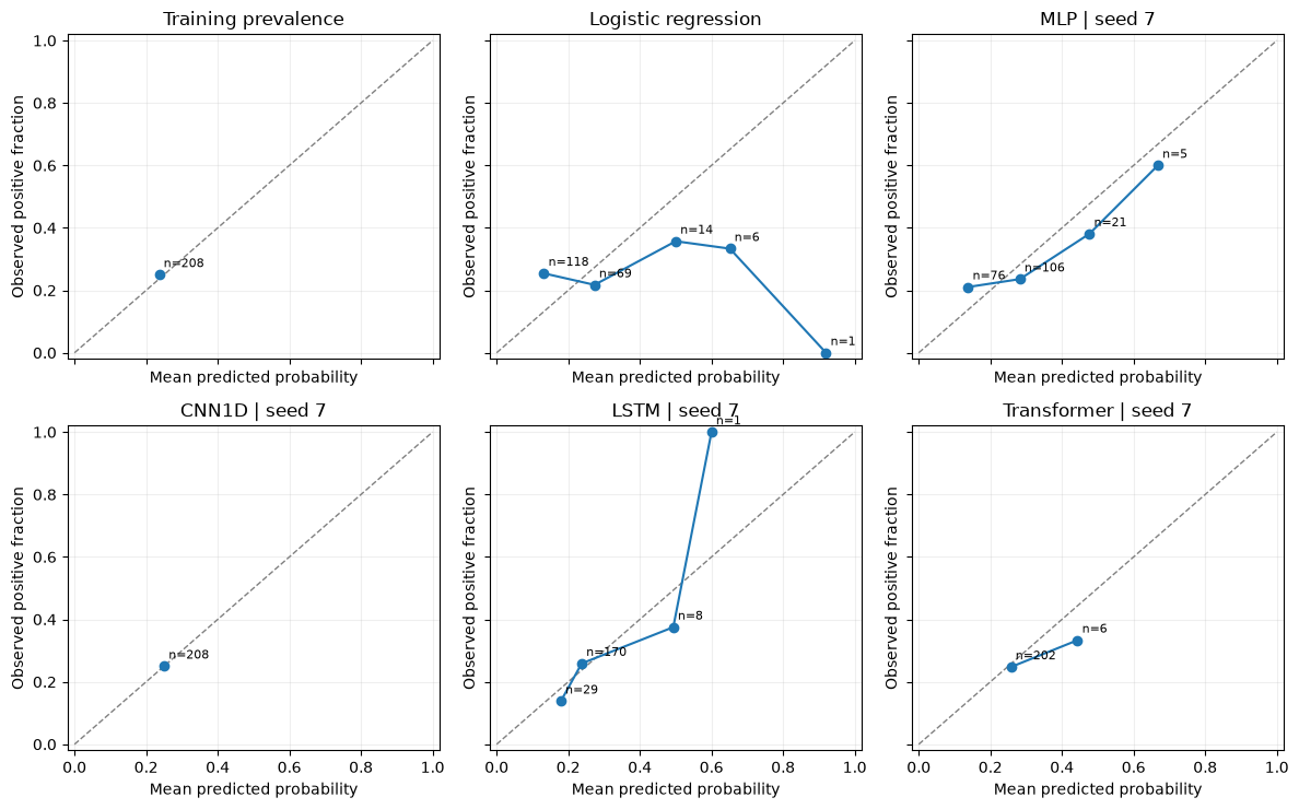
A reliability plot compares the average predicted probability with the observed positive fraction. We use five fixed bins and annotate their sample counts. Empty bins have no estimated event rate and are omitted from the lines. A point based on a handful of weeks is weak evidence about calibration.
To avoid selecting a favorable run or silently averaging predictions into an ensemble, the plots use the first predeclared seed for every neural model. The full score tables above retain all seeds. Adjacent windows share input days and seismic sequences can remain dependent, so these plots are descriptive; no independent-bin confidence intervals are claimed.
Checkpoint. Can a nearly constant forecast be well calibrated while providing little discrimination between weeks?
Live checkpoint (43-50, then 50-57). Inspect the LSTM panel with its bin counts first. At the Transformer comparison, inspect its panel using the same axes and bins. A lower Brier score alone does not establish good calibration, and a small bin cannot support a precise calibration claim.
Code block 14 · Run the matching prepared-notebook cell in order. For self-study, copy into a new Colab code cell.
def calibration_table(y_true, probabilities, bins=5):
    edges = np.linspace(0.0, 1.0, bins + 1)
    indices = np.searchsorted(edges[1:-1], probabilities, side='right')
    rows = []
    for b in range(bins):
        inside = indices == b
        count = int(inside.sum())
        rows.append({
            'bin_left': edges[b], 'bin_right': edges[b + 1], 'count': count,
            'mean_probability': float(probabilities[inside].mean()) if count else np.nan,
            'observed_fraction': float(y_true[inside].mean()) if count else np.nan,
        })
    return pd.DataFrame(rows)

calibration_frames = []
fig, axes = plt.subplots(2, 3, figsize=(12, 7.5), sharex=True, sharey=True)
for ax, name in zip(axes.flat, model_order):
    seed = SEEDS[0] if name in BUILDERS else None
    table = calibration_table(y_val, validation_predictions[(name, seed)])
    calibration_frames.append(table.assign(model=name, seed=seed))
    occupied = table[table['count'] > 0]
    ax.plot([0, 1], [0, 1], '--', color='gray', linewidth=1)
    ax.plot(occupied['mean_probability'], occupied['observed_fraction'], 'o-')
    for row in occupied.itertuples():
        ax.annotate(f'n={row.count}', (row.mean_probability, row.observed_fraction),
                    xytext=(3, 5), textcoords='offset points', fontsize=8)
    suffix = f' | seed {seed}' if seed is not None else ''
    ax.set(title=name + suffix, xlim=(-0.02, 1.02), ylim=(-0.02, 1.02),
           xlabel='Mean predicted probability', ylabel='Observed positive fraction')
    ax.grid(alpha=0.2)
plt.tight_layout()
plt.show()
calibration = pd.concat(calibration_frames, ignore_index=True)
display(calibration)
Prepared local output — expand to compare
| bin_left | bin_right | count | mean_probability | observed_fraction | model | seed | |
|---|---|---|---|---|---|---|---|
| 0 | 0.0 | 0.2 | 0 | NaN | NaN | Training prevalence | None |
| 1 | 0.2 | 0.4 | 208 | 0.236211 | 0.250000 | Training prevalence | None |
| 2 | 0.4 | 0.6 | 0 | NaN | NaN | Training prevalence | None |
| 3 | 0.6 | 0.8 | 0 | NaN | NaN | Training prevalence | None |
| 4 | 0.8 | 1.0 | 0 | NaN | NaN | Training prevalence | None |
| 5 | 0.0 | 0.2 | 118 | 0.131998 | 0.254237 | Logistic regression | None |
| 6 | 0.2 | 0.4 | 69 | 0.273292 | 0.217391 | Logistic regression | None |
| 7 | 0.4 | 0.6 | 14 | 0.500278 | 0.357143 | Logistic regression | None |
| 8 | 0.6 | 0.8 | 6 | 0.651486 | 0.333333 | Logistic regression | None |
| 9 | 0.8 | 1.0 | 1 | 0.919837 | 0.000000 | Logistic regression | None |
| 10 | 0.0 | 0.2 | 76 | 0.137772 | 0.210526 | MLP | 7 |
| 11 | 0.2 | 0.4 | 106 | 0.282319 | 0.235849 | MLP | 7 |
| 12 | 0.4 | 0.6 | 21 | 0.476655 | 0.380952 | MLP | 7 |
| 13 | 0.6 | 0.8 | 5 | 0.667842 | 0.600000 | MLP | 7 |
| 14 | 0.8 | 1.0 | 0 | NaN | NaN | MLP | 7 |
| 15 | 0.0 | 0.2 | 0 | NaN | NaN | CNN1D | 7 |
| 16 | 0.2 | 0.4 | 208 | 0.250175 | 0.250000 | CNN1D | 7 |
| 17 | 0.4 | 0.6 | 0 | NaN | NaN | CNN1D | 7 |
| 18 | 0.6 | 0.8 | 0 | NaN | NaN | CNN1D | 7 |
| 19 | 0.8 | 1.0 | 0 | NaN | NaN | CNN1D | 7 |
| 20 | 0.0 | 0.2 | 29 | 0.179272 | 0.137931 | LSTM | 7 |
| 21 | 0.2 | 0.4 | 170 | 0.237560 | 0.258824 | LSTM | 7 |
| 22 | 0.4 | 0.6 | 8 | 0.493324 | 0.375000 | LSTM | 7 |
| 23 | 0.6 | 0.8 | 1 | 0.600097 | 1.000000 | LSTM | 7 |
| 24 | 0.8 | 1.0 | 0 | NaN | NaN | LSTM | 7 |
| 25 | 0.0 | 0.2 | 0 | NaN | NaN | Transformer | 7 |
| 26 | 0.2 | 0.4 | 202 | 0.257570 | 0.247525 | Transformer | 7 |
| 27 | 0.4 | 0.6 | 6 | 0.443502 | 0.333333 | Transformer | 7 |
| 28 | 0.6 | 0.8 | 0 | NaN | NaN | Transformer | 7 |
| 29 | 0.8 | 1.0 | 0 | NaN | NaN | Transformer | 7 |
10. Save this run and state its limits
Save the validation probabilities, all seed metrics, calibration counts, training traces, and settings into this execution’s new output folder. This does not modify the frozen data or previous course results. Colab storage is temporary: download the resulting archive before closing the session.
These are retrospective development results from a revised catalogue. They do not demonstrate prospective forecasting skill, real-time catalogue availability, causation, earthquake prediction at an exact time/location, or operational warning performance.
Closing checkpoint (57-60). Complete three sentences: “Our LSTM comparison shows …”; “These validation results cannot establish …”; “The next controlled experiment would change … while keeping … fixed.” Distinguish an architecture change from a change to the input representation.
Code block 15 · Run the matching prepared-notebook cell in order. For self-study, copy into a new Colab code cell.
import shutil

TEMPORAL_RUN_DIR = RUN_DIR / 'temporal'
TEMPORAL_RUN_DIR.mkdir(parents=True, exist_ok=False)
metrics.to_csv(TEMPORAL_RUN_DIR / 'validation_metrics_by_seed.csv', index=False)
summary.to_csv(TEMPORAL_RUN_DIR / 'validation_metric_summary.csv')
pd.concat(prediction_frames, ignore_index=True).to_csv(
    TEMPORAL_RUN_DIR / 'validation_predictions.csv', index=False)
calibration.to_csv(TEMPORAL_RUN_DIR / 'validation_calibration.csv', index=False)
(TEMPORAL_RUN_DIR / 'training_histories.json').write_text(
    json.dumps(training_histories, indent=2), encoding='utf-8')
metadata = {
    'tutorial': 'temporal', 'catalogue_mode': 'revised_retrospective',
    'features': FEATURE_NAMES, 'input_shape': list(INPUT_SHAPE),
    'seeds': list(SEEDS), 'max_epochs': EPOCHS, 'batch_size': BATCH_SIZE,
    'optimizer': 'Adam', 'learning_rate': 0.001,
    'early_stopping': {'monitor': 'val_loss', 'patience': 3, 'restore_best_weights': True},
    'shuffle': False, 'scaler_fit_split': 'training',
    'validation_used_for_stopping': True, 'test_evaluated': False,
    'target': 'At least one M >= 5 catalogue event in the following seven days',
    'train_origin_range': [str(origins[train_mask][0]), str(origins[train_mask][-1])],
    'validation_origin_range': [str(validation_origins[0]), str(validation_origins[-1])],
    'training_windows': len(y_train), 'validation_windows': len(y_val),
    'training_prevalence': training_prevalence,
    'logistic': {'C': 1.0, 'penalty': 'l2', 'solver': 'lbfgs', 'max_iter': 2000},
    'tensorflow_version': tf.__version__, 'keras_version': keras.__version__,
    'numpy_version': np.__version__, 'sklearn_version': sklearn.__version__,
    'interpretation': 'Descriptive validation comparison; no independent prospective evaluation',
}
(TEMPORAL_RUN_DIR / 'run_metadata.json').write_text(
    json.dumps(metadata, indent=2), encoding='utf-8')
# Include the shared data provenance and exact window assignments in the archive.
shutil.copy2(RUN_DIR / 'protocol.json', TEMPORAL_RUN_DIR / 'data_protocol.json')
shutil.copy2(RUN_DIR / 'windows.csv', TEMPORAL_RUN_DIR / 'windows.csv')
archive = shutil.make_archive(str(RUN_DIR / 'temporal-results'), 'zip', TEMPORAL_RUN_DIR)
print('Saved:', TEMPORAL_RUN_DIR)
print('Archive:', archive)
# In Colab, uncomment these two lines to download your results:
# from google.colab import files
# files.download(archive)
Prepared local output — expand to compare
Saved: tutorial-runs\temporal-0da80b1f5731\temporal
Archive: H:\Otros ordenadores\Mi PC\1_Proyectos\2026 - Statsei 14 -\statsei14-deep-learning\qa\tutorials-2026-10-07\executions\temporal-05f6da6b\tutorial-runs\temporal-0da80b1f5731\temporal-results.zip
After class: change one thing at a time
- Complete the MLP and CNN1D explanations, then relate all four architectures to the same 30 x 3 input. Their definitions and results are already part of the sequentially executable notebook.
- Inspect which probability errors drive a difference in Brier score and log loss; use the saved predictions and every predeclared seed rather than the best-looking run.
- Plan a separate input experiment: add the same precomputed ETAS-inspired history channel to every architecture, with the same partitions and training-only scaling. Treat this as an input comparison; do not mix it with the current architecture comparison or use the historical test to choose changes.
- Continue to the spatial tutorials. A regional daily count has forgotten where the events occurred. A grid and a graph can retain location before the temporal model reads the history.
- Rebuild the notebook from a blank Colab, copying the numbered blocks in order, if you want to practice assembling the complete data and modelling pipeline yourself.
The live session remains 30 minutes of presentation plus 30 minutes of practical work: open and understand a window (30-34), references and LSTM (34-43), probability evaluation (43-50), Transformer comparison (50-57), and discussion (57-60). Prepared local outputs support the discussion if the fresh run has not finished; a real Colab run must be verified separately.
References and next steps
- Keras: Time-series classification from scratch (CNN1D)
- Keras: Time-series classification with a Transformer model
- Keras: Conv1D layer
- Keras: LSTM layer
- Keras: MultiHeadAttention layer
Return to the practical guide. These implementations adapt general Keras mechanisms to an exploratory teaching task; their documentation does not validate earthquake forecasting skill.