Deep Learning Meets ETAS
STATSEI14 · Practical tutorial
Deep Learning Meets ETAS
Practical hybrid workflows for seismic forecasting
Connect deep learning in seismology with our Spatial Statistics and aftershock research. Then follow a small LSTM from catalogue history to a weekly probability. Read its construction, training and evaluation in consecutive cells, then compare it with a compact Transformer.
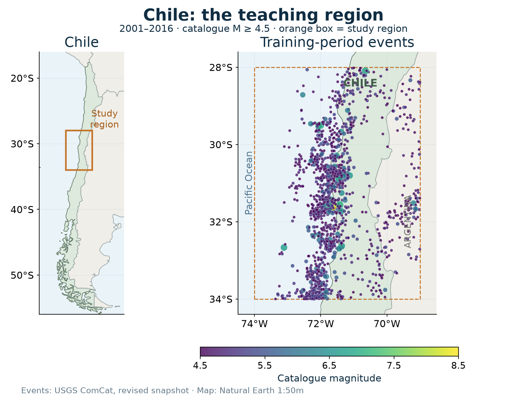
A regional catalogue becomes a sequence of forecasting examples.
Guiding question: How can flexible learning tools help us represent seismic history and investigate a clearly specified question? In the practical, that question becomes the probability of at least one catalogue event with magnitude M ≥ 5 in this region during the next seven days.
What you will be able to do
- Connect a scientific question to a representation, neural architecture, output and loss.
- Distinguish the targets in the Spatial Statistics study, the aftershock work and this practical.
- Recognize one catalogue window, run an LSTM and interpret probability scores against simple baselines.
- Explain what attention changes in a Transformer; identify maps and graphs as spatial extensions for the laboratory.
- Carry a testable question about representation or modelling into the homework.
Before the session
The session welcomes researchers with different levels of Python and deep learning experience. Basic Python helps when running or modifying cells; no previous neural-network training is required. You can also follow the prepared outputs, formulate a hypothesis and interpret the evidence with the group.
Bring a laptop and a browser if you plan to run the code. Download the prepared temporal notebook, open Colab and upload that notebook before the session. Run the core cells in order through the LSTM evaluation; the frozen catalogue downloads automatically. Each model has its own visible compile, fit and predict calls. Keep the web guide alongside it for explanations and prepared local outputs. Rebuilding the exercise in a blank notebook remains an option for independent study. The recorded execution checks are local CPU runs; a complete Colab execution remains unverified.
Thirty minutes of presentation, thirty minutes of practice
| Minutes | Activity |
|---|---|
| 00–06 | Seismic learning tasks: inputs, outputs and today’s question |
| 06–12 | A network, its loss, and a brief map of MLP, CNN, LSTM and generative learning |
| 12–18 | Spatial Statistics: how a representation defines a learning problem |
| 18–24 | Isidora’s work: how the target changes what a model can learn |
| 24–30 | One 30 × 3 window, a weekly label, baselines and chronological evaluation |
| 30–34 | Open the prepared notebook and inspect one example |
| 34–43 | Define the references; build, compile, fit and predict with the LSTM |
| 43–50 | Interpret weekly probabilities, Brier, log loss and calibration |
| 50–57 | Transformer on the same history: positional information, attention and results |
| 57–60 | Discuss one finding and choose a laboratory extension |
The first 30 minutes connect seismic applications, research cases and the practical question. The next 30 minutes cover the prepared notebook, LSTM evaluation, a Transformer comparison and discussion. MLP and CNN1D follow the live route as optional laboratory sections. The primary notebook uses seed 7 once per model so that each fit can be followed directly. A separate comparison retains seeds 7, 17 and 27. Maps, graphs and the ETAS-inspired feature experiment are follow-up routes.
Guided tutorials
- One regional sequence, step by step: references, LSTM and Transformer, with MLP and CNN1D for the laboratory.
- Sequences of maps: CNN2D + LSTM and ConvLSTM2D.
- The same cells as a graph: graph convolution + LSTM.
- All tutorials and the shared protocol.
The slides, notebook and instructor guide follow this same 30 + 30 route. The three-seed temporal comparison preserves the original repeated experiment separately. The earlier LSTM/ETAS-inspired notebooks and Transformer pilot remain a separate reference experiment. Their model definitions and scores are not the results of the current tutorial.
Session materials and laboratory extensions
- Presentation in HTML and PDF.
- Temporal notebook with ready-to-run cells.
- Temporal notebook with prepared local outputs.
- Temporal web guide and prepared results from seed 7.
- Three-seed comparison for the laboratory and its notebook.
- Complete tutorial pack: linear temporal, map and graph notebooks, separate repeated comparisons and frozen data.
- Instructor guide.
- References and source distinctions.
- Laboratory questions.
- Earlier LSTM/ETAS exercise and Transformer pilot.
The current comparison evaluates validation only, and early stopping also uses validation. An observed score difference describes this teaching experiment; it does not identify its cause or establish a general ranking of architectures. Read Brier, log loss and calibration together, and compare with training prevalence and logistic regression. The live table describes one fit per model with seed 7. It does not measure variability across initializations. Use the separate repeated comparison to examine all three declared seeds; keep its means separate from the live results.
What the experiment can establish
This is a retrospective teaching benchmark using a frozen, revised USGS catalogue. Windows exclude future event times and target intervals cannot cross split boundaries. The downloaded records do not reconstruct the catalogue versions originally available at each historical forecast time.
The ETAS-inspired score is a simplified, truncated triggering feature with illustrative parameters. It is not a fitted ETAS model. An ETAS–GAN combination remains a research proposal, outside the empirical scope of the manuscript discussed and this practical. Neither the course nor a high probability is an operational earthquake warning.