The same six cells as a graph
A linear Graph + LSTM extension
Download prepared notebook Open Colab to upload the notebook Notebook with verified local outputs Three-seed reference comparison All tutorials
Prepared outputs were verified in a fresh local kernel using the frozen data pack. They describe seed 7 individual runs, not three-seed averages. Colab execution has not been verified.
A guided Graph + LSTM example for STATSEI14
We represent the six geographic cells as nodes. Each node contains 30 days of three catalogue features. The model returns the probability of at least one catalogue event with magnitude M \geq 5 in each cell during the following seven days.
Read and run the cells in order: prepare the data, draw the graph, define the model, fit it, and inspect its probabilities. Intermediate arrays and model operations remain visible throughout.
This guided version uses seed 7 once. The complete graph tutorial retains the original three-seed experiment (7, 17, 27). A single run does not reproduce its across-seed summary or measure initialization variability.
Evaluation: training 2001–2016 and validation 2017–2020. Validation also controls early stopping, so the displayed scores are development diagnostics. We do not evaluate the previously inspected 2021–2025 test period. The catalogue is a frozen, revised record; this is a retrospective teaching experiment.
Session placement. This is a self-study extension after the 30-minute presentation and 30-minute temporal practical. The data preparation is complete and can run independently. Prepared outputs, when provided, come from a verified local run of these cells; Colab execution has not been verified.
Preparation A. Load the tools
Select a Python CPU runtime in Colab. If imports are unavailable, run %pip install tensorflow==2.19.1 keras==3.15.1 pandas scikit-learn matplotlib, restart the runtime, and begin again.
This walkthrough uses one declared seed, 7, so we can follow each fit directly. The full course guides retain three seeds (7, 17, 27). A single fit does not measure variability across initializations. The examples below generate their own results.
Code block 1 · Run the matching prepared-notebook cell in order. For self-study, copy into a new Colab code cell.
import io
import hashlib
import zipfile
import time
from pathlib import Path
from urllib.request import urlopen

import numpy as np
import pandas as pd
import matplotlib.pyplot as plt
import tensorflow as tf
from tensorflow import keras
from IPython.display import display

SEED = 7
LOOKBACK = 30
HORIZON = 7
EPOCHS = 20
BATCH_SIZE = 64

print("TensorFlow:", tf.__version__, "Keras:", keras.__version__)
Verified local output · single seed — expand to compare
TensorFlow: 2.19.1 Keras: 3.15.1
Preparation B. Read the frozen catalogue
The download is pinned to the same Git commit as the published tutorial. The two checks identify the exact ZIP and catalogue. We read only the CSV in memory, so no extraction or project-folder machinery is needed.
The catalogue contains revised records. This is a retrospective teaching exercise. We use training (2001–2016) and validation (2017–2020); the previously inspected 2021–2025 period is not evaluated here.
For offline use, upload the frozen data pack as statsei14-data-pack.zip in the working directory before running this cell. Otherwise the cell downloads the pinned ZIP. Both paths check the same SHA-256 values.
Code block 2 · Run the matching prepared-notebook cell in order. For self-study, copy into a new Colab code cell.
PACK_URL = "https://raw.githubusercontent.com/FranPlaza/FranPlaza.github.io/0e7a7e4b1c38490018f11b26170fe6a87e4997f9/courses/statsei14/downloads/data-pack.zip"
PACK_SHA256 = "0ee5d4d71aafa19023fdb1ee6f289a11e7fd7f4ed88ad7a91032ca24505d10a2"
CATALOGUE_SHA256 = "16e9b731a5b407d75a2321d3d0d2c889542e8223a9ee4fe81efe624eb6b166d2"

local_pack = Path("statsei14-data-pack.zip")
if local_pack.exists():
    pack_bytes = local_pack.read_bytes()
    print("Data source: local frozen pack")
else:
    with urlopen(PACK_URL, timeout=60) as response:
        pack_bytes = response.read()
    print("Data source: pinned download")
assert hashlib.sha256(pack_bytes).hexdigest() == PACK_SHA256

with zipfile.ZipFile(io.BytesIO(pack_bytes)) as archive:
    csv_bytes = archive.read("data/frozen/usgs_chile_2000_2025.csv")
assert hashlib.sha256(csv_bytes).hexdigest() == CATALOGUE_SHA256

events = pd.read_csv(io.BytesIO(csv_bytes))
events["time"] = pd.to_datetime(events["time"], utc=True)
events = events.sort_values("time").reset_index(drop=True)
display(events[["time", "latitude", "longitude", "mag"]].head())
Verified local output · single seed — expand to compare
Data source: local frozen pack
| time | latitude | longitude | mag | |
|---|---|---|---|---|
| 0 | 2000-01-07 11:49:11.720000+00:00 | -28.495 | -69.196 | 4.0 |
| 1 | 2000-01-08 11:43:58.150000+00:00 | -31.017 | -71.339 | 4.4 |
| 2 | 2000-01-11 13:16:34.420000+00:00 | -30.747 | -71.319 | 4.5 |
| 3 | 2000-01-18 17:12:18.360000+00:00 | -31.630 | -71.451 | 4.9 |
| 4 | 2000-01-19 01:24:00.150000+00:00 | -31.440 | -71.384 | 3.8 |
Preparation C. Select the region and define the daily calendar
Input events satisfy M ≥ 4.5. The future occurrence target uses M ≥ 5. We retain every calendar day, including days without events. The first year supplies history for the earliest training windows.
The three channels are log(1 + count), maximum magnitude excess above 4.5, and presence. Presence distinguishes an empty day from a day containing an event exactly at the input threshold.
Code block 3 · Run the matching prepared-notebook cell in order. For self-study, copy into a new Colab code cell.
START = pd.Timestamp("2000-01-01", tz="UTC")
END = pd.Timestamp("2026-01-01", tz="UTC")
days = pd.date_range(START, END - pd.Timedelta(days=1), freq="D")
FEATURES = ["log_count", "max_magnitude_excess", "has_event"]

inside = events["latitude"].between(-34.0, -28.0)
inside &= events["longitude"].between(-74.0, -69.0)
in_time = (events["time"] >= START) & (events["time"] < END)
selected = events.loc[inside & in_time & (events["mag"] >= 4.5)].copy()
selected["date"] = selected["time"].dt.floor("D")
print("Input events:", len(selected))
Verified local output · single seed — expand to compare
Input events: 2121
Preparation D. Keep the same six geographic cells
Three latitude bands and two longitude bands form a 3 × 2 grid. Row zero is south; column zero is west. A boundary event goes into the cell to its north/east, except at the outer boundary, where it stays in the last cell. These are geographic bins, not fitted tectonic provinces.
The group index lists every day and every cell. Reindexing inserts empty combinations before reshaping them into maps.
Code block 4 · Run the matching prepared-notebook cell in order. For self-study, copy into a new Colab code cell.
LAT_EDGES = np.array([-34.0, -32.0, -30.0, -28.0])
LON_EDGES = np.array([-74.0, -71.5, -69.0])
N_ROWS, N_COLS = 3, 2

selected["row"] = np.searchsorted(LAT_EDGES, selected["latitude"], side="right") - 1
selected["col"] = np.searchsorted(LON_EDGES, selected["longitude"], side="right") - 1
selected["row"] = selected["row"].clip(0, N_ROWS - 1)
selected["col"] = selected["col"].clip(0, N_COLS - 1)

cell_index = pd.MultiIndex.from_product(
    [days, range(N_ROWS), range(N_COLS)], names=["date", "row", "col"]
)
grouped = selected.groupby(["date", "row", "col"])
counts = grouped.size().reindex(cell_index, fill_value=0)
counts = counts.to_numpy(dtype="float32").reshape(len(days), N_ROWS, N_COLS)

max_excess = (grouped["mag"].max() - 4.5).reindex(cell_index, fill_value=0)
max_excess = max_excess.to_numpy(dtype="float32").reshape(len(days), N_ROWS, N_COLS)

larger_events = selected.loc[selected["mag"] >= 5.0]
target_counts = larger_events.groupby(["date", "row", "col"]).size()
target_counts = target_counts.reindex(cell_index, fill_value=0)
target_counts = target_counts.to_numpy(dtype="float32").reshape(len(days), N_ROWS, N_COLS)

daily_grid_raw = np.stack([
    np.log1p(counts), max_excess, (counts > 0).astype("float32")
], axis=-1).astype("float32")
assert counts.sum() == len(selected)
print("Daily maps (days, rows, columns, channels):", daily_grid_raw.shape)
Verified local output · single seed — expand to compare
Daily maps (days, rows, columns, channels): (9497, 3, 2, 3)
Preparation E. One Monday becomes one learning example
At origin t, take inputs from [t − 30 days, t) and the outcome from [t, t + 7 days). The Python slices below implement those intervals directly. We omit target weeks that cross a partition boundary.
Only origins through 2020 are built. The retained examples are the same training and validation examples as in the original guide. Weekly targets do not overlap, although input histories share days.
Code block 5 · Run the matching prepared-notebook cell in order. For self-study, copy into a new Colab code cell.
VAL_START = pd.Timestamp("2017-01-01", tz="UTC")
TEST_START = pd.Timestamp("2021-01-01", tz="UTC")
candidate_origins = pd.date_range("2001-01-01", "2020-12-31", freq="W-MON", tz="UTC")

histories, outcomes, kept_origins = [], [], []
for origin in candidate_origins:
    i = days.get_loc(origin)
    target_end = origin + pd.Timedelta(days=HORIZON)
    boundary = VAL_START if origin < VAL_START else TEST_START
    if i < LOOKBACK or target_end > boundary:
        continue

    history = daily_grid_raw[i - LOOKBACK:i]
    future_counts = target_counts[i:i + HORIZON]
    outcome = (future_counts.sum(axis=0) > 0).astype("int32")
    histories.append(history)
    outcomes.append(outcome)
    kept_origins.append(origin)

origins = pd.DatetimeIndex(kept_origins)
raw_grid = np.stack(histories)
y_grid = np.asarray(outcomes, dtype="int32")
train_mask = origins < VAL_START
val_mask = origins >= VAL_START

assert (origins[train_mask] + pd.Timedelta(days=HORIZON) <= VAL_START).all()
assert (origins[val_mask] + pd.Timedelta(days=HORIZON) <= TEST_START).all()
print("Training examples:", train_mask.sum(), "Validation examples:", val_mask.sum())
print("One input:", raw_grid[0].shape, "One outcome:", y_grid[0])
Verified local output · single seed — expand to compare
Training examples: 834 Validation examples: 208
One input: (30, 3, 2, 3) One outcome: [[1 0]
 [1 0]
 [0 0]]
Preparation F. Estimate scaling from training histories
There is one mean and one standard deviation per channel. For maps, cells share these scaling parameters. We keep the original weighting over overlapping training windows. Validation has no role in estimating these parameters.
Code block 6 · Run the matching prepared-notebook cell in order. For self-study, copy into a new Colab code cell.
grid_mean = raw_grid[train_mask].mean(axis=(0, 1, 2, 3), dtype=np.float64)
grid_scale = raw_grid[train_mask].std(axis=(0, 1, 2, 3), dtype=np.float64)
grid_scale = np.where(grid_scale > 0, grid_scale, 1.0)
X_grid = ((raw_grid - grid_mean) / grid_scale).astype("float32")
assert np.isfinite(X_grid).all()

display(pd.DataFrame({
    "channel": FEATURES, "training_mean": grid_mean, "training_sd": grid_scale
}))
Verified local output · single seed — expand to compare
| channel | training_mean | training_sd | |
|---|---|---|---|
| 0 | log_count | 0.022593 | 0.142629 |
| 1 | max_magnitude_excess | 0.010133 | 0.094568 |
| 2 | has_event | 0.028624 | 0.166747 |
Represent the six cells as nodes
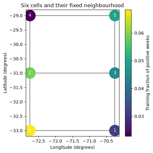
A node is a geographic cell, not an earthquake or a seismic station. Number cells west to east within each row, then south to north. Reshaping the grid preserves that order in the inputs and targets.
- Grid sample:
(30 days, 3 rows, 2 columns, 3 features). - Graph sample:
(30 days, 6 nodes, 3 features). - Target: six binary outcomes for the next seven days.
Several cells may be positive in the same week. The six probabilities therefore need not sum to one. These are illustrative geographic bins, with different physical areas, rather than inferred tectonic regions.
Code block 7 · Run the matching prepared-notebook cell in order. For self-study, copy into a new Colab code cell.
N_NODES = N_ROWS * N_COLS

X_nodes = X_grid.reshape(len(X_grid), LOOKBACK, N_NODES, len(FEATURES))
Y_nodes = y_grid.reshape(len(y_grid), N_NODES).astype("float32")

X_train = X_nodes[train_mask]
X_val = X_nodes[val_mask]
y_train = Y_nodes[train_mask]
y_val = Y_nodes[val_mask]
validation_origins = origins[val_mask]

# Node 0 is the southwest cell in both arrays.
assert np.array_equal(X_nodes[:, :, 0], X_grid[:, :, 0, 0])
assert np.array_equal(Y_nodes[:, 0], y_grid[:, 0, 0])

lat_centres = (LAT_EDGES[:-1] + LAT_EDGES[1:]) / 2
lon_centres = (LON_EDGES[:-1] + LON_EDGES[1:]) / 2
node_table = pd.DataFrame({
    "node": np.arange(N_NODES),
    "row": np.repeat(np.arange(N_ROWS), N_COLS),
    "column": np.tile(np.arange(N_COLS), N_ROWS),
    "latitude": np.repeat(lat_centres, N_COLS),
    "longitude": np.tile(lon_centres, N_ROWS),
    "training_positive_weeks": y_train.sum(axis=0).astype(int),
    "training_prevalence": y_train.mean(axis=0),
})

display(node_table)
print("Training:", X_train.shape, "targets:", y_train.shape)
print("Validation:", X_val.shape, "targets:", y_val.shape)
Verified local output · single seed — expand to compare
| node | row | column | latitude | longitude | training_positive_weeks | training_prevalence | |
|---|---|---|---|---|---|---|---|
| 0 | 0 | 0 | 0 | -33.0 | -72.75 | 57 | 0.068345 |
| 1 | 1 | 0 | 1 | -33.0 | -70.25 | 26 | 0.031175 |
| 2 | 2 | 1 | 0 | -31.0 | -72.75 | 49 | 0.058753 |
| 3 | 3 | 1 | 1 | -31.0 | -70.25 | 37 | 0.044365 |
| 4 | 4 | 2 | 0 | -29.0 | -72.75 | 19 | 0.022782 |
| 5 | 5 | 2 | 1 | -29.0 | -70.25 | 41 | 0.049161 |
Training: (834, 30, 6, 3) targets: (834, 6)
Validation: (208, 30, 6, 3) targets: (208, 6)
Connect neighbouring cells
Join cells that share an edge, without diagonal connections. The adjacency matrix A[i, j] is 1 when cells i and j are neighbours. Add a self-loop and divide each row by its total. Multiplication by A_normalized then averages each node’s features with those of its immediate neighbours.
This geometric graph is fixed before modelling. An edge specifies an information-sharing rule; it does not establish physical triggering between cells.
Code block 8 · Run the matching prepared-notebook cell in order. For self-study, copy into a new Colab code cell.
A = np.zeros((N_NODES, N_NODES), dtype="float32")

# The six cells have these seven undirected edges.
edges = [(0, 1), (0, 2), (1, 3), (2, 3), (2, 4), (3, 5), (4, 5)]
for i, j in edges:
    A[i, j] = 1
    A[j, i] = 1

A_with_self = A + np.eye(N_NODES, dtype="float32")
A_normalized = A_with_self / A_with_self.sum(axis=1, keepdims=True)

assert np.array_equal(A, A.T)
assert np.allclose(A_normalized.sum(axis=1), 1)
display(pd.DataFrame(A_normalized, index=range(N_NODES), columns=range(N_NODES)))
Verified local output · single seed — expand to compare
| 0 | 1 | 2 | 3 | 4 | 5 | |
|---|---|---|---|---|---|---|
| 0 | 0.333333 | 0.333333 | 0.333333 | 0.000000 | 0.000000 | 0.000000 |
| 1 | 0.333333 | 0.333333 | 0.000000 | 0.333333 | 0.000000 | 0.000000 |
| 2 | 0.250000 | 0.000000 | 0.250000 | 0.250000 | 0.250000 | 0.000000 |
| 3 | 0.000000 | 0.250000 | 0.250000 | 0.250000 | 0.000000 | 0.250000 |
| 4 | 0.000000 | 0.000000 | 0.333333 | 0.000000 | 0.333333 | 0.333333 |
| 5 | 0.000000 | 0.000000 | 0.000000 | 0.333333 | 0.333333 | 0.333333 |
Code block 9 · Run the matching prepared-notebook cell in order. For self-study, copy into a new Colab code cell.
fig, ax = plt.subplots(figsize=(5, 5))

# Draw each undirected edge once.
for i, j in zip(*np.where(np.triu(A, k=1))):
    ax.plot(node_table.loc[[i, j], "longitude"],
            node_table.loc[[i, j], "latitude"], color="grey", zorder=1)

points = ax.scatter(node_table.longitude, node_table.latitude,
                    c=node_table.training_prevalence, s=650,
                    cmap="viridis", zorder=2)
for node in node_table.itertuples():
    ax.text(node.longitude, node.latitude, str(node.node),
            ha="center", va="center", color="white")

ax.set(xlabel="Longitude (degrees)", ylabel="Latitude (degrees)",
       title="Six cells and their fixed neighbourhood")
fig.colorbar(points, ax=ax, label="Training fraction of positive weeks")
fig.tight_layout()
plt.show()
Verified local output · single seed — expand to compare
Inspect one message-passing step
Before learning any weights, inspect the averaging operation on the last day of the first training window. Every row still refers to the same node. These are standardized feature values, not event counts.
Check node 0 in the adjacency table: its average includes nodes 0, 1 and 2. A single graph layer cannot transmit a message across two edges.
Code block 10 · Run the matching prepared-notebook cell in order. For self-study, copy into a new Colab code cell.
one_day = X_train[0, -1]                 # (6 nodes, 3 features)
neighbour_mean = A_normalized @ one_day  # The same shape, after averaging.

display(pd.DataFrame(one_day, columns=FEATURES).rename_axis("node"))
display(pd.DataFrame(neighbour_mean, columns=FEATURES).rename_axis("node"))
print("Node 0 mean:", one_day[[0, 1, 2]].mean(axis=0))
Verified local output · single seed — expand to compare
| log_count | max_magnitude_excess | has_event | |
|---|---|---|---|
| node | |||
| 0 | -0.158405 | -0.107146 | -0.17166 |
| 1 | -0.158405 | -0.107146 | -0.17166 |
| 2 | -0.158405 | -0.107146 | -0.17166 |
| 3 | -0.158405 | -0.107146 | -0.17166 |
| 4 | -0.158405 | -0.107146 | -0.17166 |
| 5 | -0.158405 | -0.107146 | -0.17166 |
| log_count | max_magnitude_excess | has_event | |
|---|---|---|---|
| node | |||
| 0 | -0.158405 | -0.107146 | -0.17166 |
| 1 | -0.158405 | -0.107146 | -0.17166 |
| 2 | -0.158405 | -0.107146 | -0.17166 |
| 3 | -0.158405 | -0.107146 | -0.17166 |
| 4 | -0.158405 | -0.107146 | -0.17166 |
| 5 | -0.158405 | -0.107146 | -0.17166 |
Node 0 mean: [-0.1584049 -0.10714584 -0.17166023]
Define the graph convolution
The graph layer learns two transformations: one for a node’s own features and another for its neighbourhood average. Their sum passes through ReLU:
h_i = \operatorname{ReLU}\left( W_{\mathrm{self}}x_i + W_{\mathrm{neighbour}}\sum_j \overline A_{ij}x_j + b \right).
The same operation is applied at every day and node. The neighbourhood average includes the node itself; its separate self-projection is also retained, as in the complete tutorial.
This is the notebook’s only custom class. build creates the fixed adjacency weight, while call shows the graph calculation. The dense weights are learned; the adjacency matrix is not.
Code block 11 · Run the matching prepared-notebook cell in order. For self-study, copy into a new Colab code cell.
class GraphConv(keras.layers.Layer):
    def __init__(self, units, adjacency, **kwargs):
        super().__init__(**kwargs)
        self.adjacency_values = np.asarray(adjacency, dtype="float32")
        self.self_projection = keras.layers.Dense(units, use_bias=True)
        self.neighbour_projection = keras.layers.Dense(units, use_bias=False)

    def build(self, input_shape):
        self.adjacency = self.add_weight(
            name="fixed_adjacency", shape=self.adjacency_values.shape,
            initializer=keras.initializers.Constant(self.adjacency_values),
            trainable=False,
        )
        self.self_projection.build(input_shape)
        self.neighbour_projection.build(input_shape)
        super().build(input_shape)

    def call(self, inputs):
        # i receives from j; b = batch, t = time, f = feature.
        neighbour_mean = keras.ops.einsum("ij,btjf->btif", self.adjacency, inputs)
        own_part = self.self_projection(inputs)
        neighbour_part = self.neighbour_projection(neighbour_mean)
        return keras.ops.relu(own_part + neighbour_part)
Combine graph messages with temporal memory
After graph convolution, put the node axis before the time axis. TimeDistributed(LSTM) applies one shared LSTM to each node’s 30-day history. A shared sigmoid head returns one probability per node.
| Stage | Shape of one sample |
|---|---|
| Input | 30 days × 6 nodes × 3 features |
| Graph convolution | 30 days × 6 nodes × 8 learned features |
| Reorder axes | 6 nodes × 30 days × 8 learned features |
| Shared LSTM | 6 nodes × 16 state values |
| Shared sigmoid head | 6 probabilities |
The head has no separate intercept for each cell. Predictions must arise from local and neighbouring histories, so compare them with each cell’s training prevalence.
Code block 12 · Run the matching prepared-notebook cell in order. For self-study, copy into a new Colab code cell.
keras.backend.clear_session()
keras.utils.set_random_seed(SEED)

inputs = keras.Input(shape=(LOOKBACK, N_NODES, len(FEATURES)),
                     name="node_sequences")
messages = GraphConv(8, A_normalized, name="spatial_messages")(inputs)
node_histories = keras.layers.Permute((2, 1, 3),
                                     name="one_sequence_per_node")(messages)
node_states = keras.layers.TimeDistributed(
    keras.layers.LSTM(16), name="shared_node_memory",
)(node_histories)
node_outputs = keras.layers.TimeDistributed(
    keras.layers.Dense(1, activation="sigmoid"),
    name="shared_probability_head",
)(node_states)
outputs = keras.layers.Reshape((N_NODES,), name="node_probabilities")(node_outputs)

model = keras.Model(inputs, outputs, name="graph_lstm")
model.compile(optimizer=keras.optimizers.Adam(learning_rate=1e-3),
              loss="binary_crossentropy")
model.summary()
assert model.output_shape == (None, N_NODES)
Verified local output · single seed — expand to compare
WARNING:tensorflow:From C:\Users\Francisco Plaza\AppData\Local\Temp\statsei14-transformer-pilot-20261007\Lib\site-packages\keras\src\backend\common\global_state.py:82: The name tf.reset_default_graph is deprecated. Please use tf.compat.v1.reset_default_graph instead.
Model: "graph_lstm"
┏━━━━━━━━━━━━━━━━━━━━━━━━━━━━━━━━━┳━━━━━━━━━━━━━━━━━━━━━━━━┳━━━━━━━━━━━━━━━┓
┃ Layer (type)                    ┃ Output Shape           ┃       Param # ┃
┡━━━━━━━━━━━━━━━━━━━━━━━━━━━━━━━━━╇━━━━━━━━━━━━━━━━━━━━━━━━╇━━━━━━━━━━━━━━━┩
│ node_sequences (InputLayer)     │ (None, 30, 6, 3)       │             0 │
├─────────────────────────────────┼────────────────────────┼───────────────┤
│ spatial_messages (GraphConv)    │ (None, 30, 6, 8)       │            92 │
├─────────────────────────────────┼────────────────────────┼───────────────┤
│ one_sequence_per_node (Permute) │ (None, 6, 30, 8)       │             0 │
├─────────────────────────────────┼────────────────────────┼───────────────┤
│ shared_node_memory              │ (None, 6, 16)          │         1,600 │
│ (TimeDistributed)               │                        │               │
├─────────────────────────────────┼────────────────────────┼───────────────┤
│ shared_probability_head         │ (None, 6, 1)           │            17 │
│ (TimeDistributed)               │                        │               │
├─────────────────────────────────┼────────────────────────┼───────────────┤
│ node_probabilities (Reshape)    │ (None, 6)              │             0 │
└─────────────────────────────────┴────────────────────────┴───────────────┘
Total params: 1,709 (6.68 KB)
Trainable params: 1,673 (6.54 KB)
Non-trainable params: 36 (144.00 B)
Establish a reference probability for each cell
For every validation week, the baseline predicts that cell’s positive fraction in the training data. It accounts for persistent differences between cells without using their validation outcomes for fitting.
Code block 13 · Run the matching prepared-notebook cell in order. For self-study, copy into a new Colab code cell.
prevalence = y_train.mean(axis=0)
p_baseline = np.tile(prevalence, (len(y_val), 1))

display(pd.DataFrame({"node": np.arange(N_NODES),
                      "baseline_probability": prevalence}))
Verified local output · single seed — expand to compare
| node | baseline_probability | |
|---|---|---|
| 0 | 0 | 0.068345 |
| 1 | 1 | 0.031175 |
| 2 | 2 | 0.058753 |
| 3 | 3 | 0.044365 |
| 4 | 4 | 0.022782 |
| 5 | 5 | 0.049161 |
Fit the model once
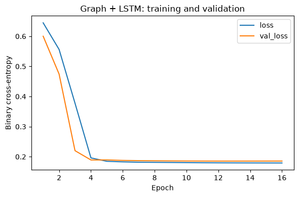
We use seed 7, a maximum of 20 epochs, batches of 64, and patience 3. Early stopping restores the weights from the lowest validation loss. The LSTM state restarts for every input window; it is not carried from training into validation examples.
A single seed makes the workflow easier to follow. Repetition across seeds belongs to the full experiment and should not be replaced by selecting the best-looking run.
Code block 14 · Run the matching prepared-notebook cell in order. For self-study, copy into a new Colab code cell.
early_stopping = keras.callbacks.EarlyStopping(
    monitor="val_loss", patience=3, restore_best_weights=True,
)

start = time.perf_counter()
history = model.fit(
    X_train, y_train,
    validation_data=(X_val, y_val),
    epochs=EPOCHS, batch_size=BATCH_SIZE, shuffle=False,
    callbacks=[early_stopping], verbose=2,
)
fit_seconds = time.perf_counter() - start

p_graph = model.predict(X_val, batch_size=BATCH_SIZE, verbose=0)
assert p_graph.shape == y_val.shape
assert np.isfinite(p_graph).all() and ((p_graph >= 0) & (p_graph <= 1)).all()
print("Validation probabilities:", p_graph.shape)
Verified local output · single seed — expand to compare
Epoch 1/20
14/14 - 3s - 195ms/step - loss: 0.6446 - val_loss: 0.6001
Epoch 2/20
14/14 - 0s - 12ms/step - loss: 0.5562 - val_loss: 0.4744
Epoch 3/20
14/14 - 0s - 12ms/step - loss: 0.3776 - val_loss: 0.2200
Epoch 4/20
14/14 - 0s - 12ms/step - loss: 0.1961 - val_loss: 0.1892
Epoch 5/20
14/14 - 0s - 13ms/step - loss: 0.1847 - val_loss: 0.1894
Epoch 6/20
14/14 - 0s - 13ms/step - loss: 0.1829 - val_loss: 0.1877
Epoch 7/20
14/14 - 0s - 12ms/step - loss: 0.1817 - val_loss: 0.1869
Epoch 8/20
14/14 - 0s - 12ms/step - loss: 0.1813 - val_loss: 0.1864
Epoch 9/20
14/14 - 0s - 12ms/step - loss: 0.1808 - val_loss: 0.1860
Epoch 10/20
14/14 - 0s - 12ms/step - loss: 0.1804 - val_loss: 0.1857
Epoch 11/20
14/14 - 0s - 12ms/step - loss: 0.1800 - val_loss: 0.1855
Epoch 12/20
14/14 - 0s - 13ms/step - loss: 0.1797 - val_loss: 0.1854
Epoch 13/20
14/14 - 0s - 12ms/step - loss: 0.1795 - val_loss: 0.1854
Epoch 14/20
14/14 - 0s - 12ms/step - loss: 0.1794 - val_loss: 0.1855
Epoch 15/20
14/14 - 0s - 12ms/step - loss: 0.1793 - val_loss: 0.1855
Epoch 16/20
14/14 - 0s - 12ms/step - loss: 0.1792 - val_loss: 0.1856
Validation probabilities: (208, 6)
Code block 15 · Run the matching prepared-notebook cell in order. For self-study, copy into a new Colab code cell.
training_history = pd.DataFrame(history.history)
training_history.index = np.arange(1, len(training_history) + 1)
training_history.index.name = "epoch"

ax = training_history[["loss", "val_loss"]].plot(figsize=(6, 4))
ax.set(xlabel="Epoch", ylabel="Binary cross-entropy",
       title="Graph + LSTM: training and validation")
plt.tight_layout()
plt.show()
Verified local output · single seed — expand to compare
Compare probability errors
Brier score is the mean squared error of probabilities. Log loss penalizes confident wrong probabilities strongly. Lower values are better for both. Clipping below is only for numerical stability in the logarithm.
Pooled scores average over all validation origins and cells. They describe six marginal probability forecasts, not a joint spatial likelihood.
Code block 16 · Run the matching prepared-notebook cell in order. For self-study, copy into a new Colab code cell.
brier_baseline = np.mean((p_baseline - y_val) ** 2)
brier_graph = np.mean((p_graph - y_val) ** 2)

baseline_clipped = np.clip(p_baseline, 1e-7, 1 - 1e-7)
graph_clipped = np.clip(p_graph, 1e-7, 1 - 1e-7)
logloss_baseline = -np.mean(
    y_val * np.log(baseline_clipped) + (1 - y_val) * np.log1p(-baseline_clipped)
)
logloss_graph = -np.mean(
    y_val * np.log(graph_clipped) + (1 - y_val) * np.log1p(-graph_clipped)
)

results = pd.DataFrame({
    "model": ["Cell prevalence", "Graph + LSTM"],
    "seed": [None, SEED],
    "validation_brier": [brier_baseline, brier_graph],
    "validation_log_loss": [logloss_baseline, logloss_graph],
    "total_parameters": [0, model.count_params()],
    "epochs": [0, len(training_history)],
    "fit_seconds": [0.0, fit_seconds],
})
display(results)
Verified local output · single seed — expand to compare
| model | seed | validation_brier | validation_log_loss | total_parameters | epochs | fit_seconds | |
|---|---|---|---|---|---|---|---|
| 0 | Cell prevalence | NaN | 0.045091 | 0.191246 | 0 | 0 | 0.000000 |
| 1 | Graph + LSTM | 7.0 | 0.043962 | 0.185415 | 1709 | 16 | 5.372494 |
The model has 1,673 trainable parameters and 36 fixed adjacency entries: 1,709 parameters in model.count_params(). These counts describe this architecture; runtime also depends on the device and stopping epoch.
Compare individual cells before interpreting the pooled score. Positive weeks are sparse, and a favourable pooled average may conceal poor results in a particular cell.
Code block 17 · Run the matching prepared-notebook cell in order. For self-study, copy into a new Colab code cell.
cell_results = node_table[["node", "latitude", "longitude"]].copy()
cell_results["validation_positive_weeks"] = y_val.sum(axis=0).astype(int)
cell_results["baseline_brier"] = np.mean((p_baseline - y_val) ** 2, axis=0)
cell_results["graph_brier"] = np.mean((p_graph - y_val) ** 2, axis=0)
cell_results["baseline_log_loss"] = -np.mean(
    y_val * np.log(baseline_clipped) + (1 - y_val) * np.log1p(-baseline_clipped), axis=0
)
cell_results["graph_log_loss"] = -np.mean(
    y_val * np.log(graph_clipped) + (1 - y_val) * np.log1p(-graph_clipped), axis=0
)
display(cell_results)
Verified local output · single seed — expand to compare
| node | latitude | longitude | validation_positive_weeks | baseline_brier | graph_brier | baseline_log_loss | graph_log_loss | |
|---|---|---|---|---|---|---|---|---|
| 0 | 0 | -33.0 | -72.75 | 10 | 0.046176 | 0.042147 | 0.196389 | 0.175586 |
| 1 | 1 | -33.0 | -70.25 | 6 | 0.028019 | 0.028519 | 0.130800 | 0.135804 |
| 2 | 2 | -31.0 | -72.75 | 14 | 0.062851 | 0.063232 | 0.247252 | 0.253526 |
| 3 | 3 | -31.0 | -70.25 | 13 | 0.058923 | 0.057101 | 0.237250 | 0.231150 |
| 4 | 4 | -29.0 | -72.75 | 9 | 0.041817 | 0.040863 | 0.185683 | 0.172534 |
| 5 | 5 | -29.0 | -70.25 | 7 | 0.032762 | 0.031912 | 0.150101 | 0.143892 |
Put the probabilities back on the map
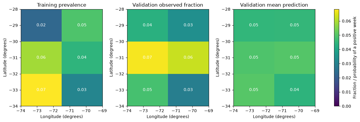
The three panels share a colour scale. Compare the training baseline, observed validation fraction, and average predicted probability. A mean map describes long-run spatial differences across these weeks; it does not show a forecast for one particular week.
Ask whether the shared graph model reproduces different cell prevalences. The probabilities describe recorded event occurrence, not shaking or risk.
Code block 18 · Run the matching prepared-notebook cell in order. For self-study, copy into a new Colab code cell.
map_fields = [
    prevalence.reshape(N_ROWS, N_COLS),
    y_val.mean(axis=0).reshape(N_ROWS, N_COLS),
    p_graph.mean(axis=0).reshape(N_ROWS, N_COLS),
]
titles = ["Training prevalence", "Validation observed fraction",
          "Validation mean prediction"]
vmax = max(float(field.max()) for field in map_fields)

fig, axes = plt.subplots(1, 3, figsize=(12, 4), constrained_layout=True)
for ax, field, title in zip(axes, map_fields, titles):
    mesh = ax.pcolormesh(LON_EDGES, LAT_EDGES, field, vmin=0,
                         vmax=max(vmax, 0.01), cmap="viridis", shading="flat")
    for node in range(N_NODES):
        row, col = divmod(node, N_COLS)
        ax.text(lon_centres[col], lat_centres[row], f"{field[row, col]:.2f}",
                ha="center", va="center", color="white")
    ax.set(title=title, xlabel="Longitude (degrees)", ylabel="Latitude (degrees)")

fig.colorbar(mesh, ax=axes, label="Fraction / probability of a positive week")
plt.show()
Verified local output · single seed — expand to compare
Optional: inspect calibration
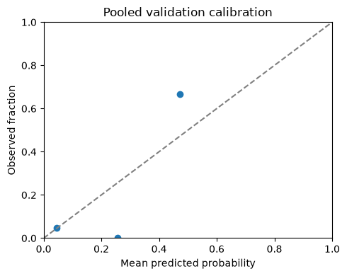
Group predictions into five fixed bins and compare their mean probability with the observed event fraction. Keep bin counts visible. Many probabilities may fall in one bin because weekly cell events are uncommon; empty bins provide no calibration information.
This pooled diagnostic combines cells and dependent histories. A small apparent discrepancy is not evidence of calibration on new data.
Code block 19 · Run the matching prepared-notebook cell in order. For self-study, copy into a new Colab code cell.
calibration_pairs = pd.DataFrame({
    "probability": p_graph.ravel(),
    "observed": y_val.ravel(),
})
calibration_pairs["bin"] = pd.cut(
    calibration_pairs.probability,
    bins=np.linspace(0, 1, 6), include_lowest=True,
)
calibration = calibration_pairs.groupby("bin", observed=True).agg(
    origin_cell_pairs=("observed", "size"),
    positives=("observed", "sum"),
    mean_probability=("probability", "mean"),
    observed_fraction=("observed", "mean"),
).reset_index()
display(calibration)

fig, ax = plt.subplots(figsize=(5, 4))
ax.plot([0, 1], [0, 1], "--", color="grey")
ax.scatter(calibration.mean_probability, calibration.observed_fraction)
ax.set(xlim=(0, 1), ylim=(0, 1), xlabel="Mean predicted probability",
       ylabel="Observed fraction", title="Pooled validation calibration")
fig.tight_layout()
plt.show()
Verified local output · single seed — expand to compare
| bin | origin_cell_pairs | positives | mean_probability | observed_fraction | |
|---|---|---|---|---|---|
| 0 | (-0.001, 0.2] | 1242 | 57.0 | 0.045836 | 0.045894 |
| 1 | (0.2, 0.4] | 3 | 0.0 | 0.257015 | 0.000000 |
| 2 | (0.4, 0.6] | 3 | 2.0 | 0.471467 | 0.666667 |
Save the tables from this run
Save scores, the training history, and one row per validation origin and node. Each prediction remains paired with its cell and observed outcome. Rerunning this cell replaces these CSV files in outputs_graphs.
Code block 20 · Run the matching prepared-notebook cell in order. For self-study, copy into a new Colab code cell.
output_dir = Path("outputs_graphs")
output_dir.mkdir(exist_ok=True)

predictions = pd.DataFrame({
    "origin": np.repeat(validation_origins.astype(str), N_NODES),
    "node": np.tile(np.arange(N_NODES), len(y_val)),
    "observed": y_val.astype(int).ravel(),
    "baseline_probability": p_baseline.ravel(),
    "graph_probability": p_graph.ravel(),
    "seed": SEED,
})

results.to_csv(output_dir / "validation_metrics.csv", index=False)
cell_results.to_csv(output_dir / "validation_metrics_by_cell.csv", index=False)
predictions.to_csv(output_dir / "validation_predictions.csv", index=False)
training_history.to_csv(output_dir / "training_history.csv")
print("Tables saved to:", output_dir.resolve())

protocol = pd.DataFrame([{
    "seed": SEED, "lookback_days": LOOKBACK, "horizon_days": HORIZON,
    "train_start": "2001-01-01", "train_end_exclusive": "2017-01-01",
    "validation_start": "2017-01-01", "validation_end_exclusive": "2021-01-01",
    "training_examples": int(train_mask.sum()), "validation_examples": int(val_mask.sum()),
    "maximum_epochs": EPOCHS, "batch_size": BATCH_SIZE, "early_stopping_patience": 3,
    "pack_sha256": PACK_SHA256, "catalogue_sha256": CATALOGUE_SHA256,
    "tensorflow_version": tf.__version__, "keras_version": keras.__version__,
    "historical_as_of_verified": False, "colab_execution_verified": False,
}])
protocol.to_csv(output_dir / "protocol.csv", index=False)
Verified local output · single seed — expand to compare
Tables saved to: H:\Otros ordenadores\Mi PC\1_Proyectos\2026 - Statsei 14 -\statsei14-deep-learning\qa\linear-integration-2026-10-07\executions\graphs-8b429cdb1b\outputs_graphs
What did the graph add?
Follow the information through the model: daily node features, neighbour averages, learned graph features, node histories, then weekly probabilities. Changing the graph changes which histories can contribute to a prediction.
A useful next experiment compares this declared graph with an identity adjacency matrix, keeping data, targets, training budget and evaluation unchanged. Repeat the predeclared seeds and retain every run. Such a control investigates the contribution of neighbour messages; the current single run cannot establish their value.
The map tutorial uses the same six cells, inputs and target windows. Its spatial scores can be compared under the same evaluation protocol. Regional tutorial scores concern a different target and should not be ranked against these cell scores.
Sources
- Original STATSEI14 graph tutorial: catalogue protocol, graph equation, architecture and full three-seed experiment.
- Keras graph and LSTM example: motivation for combining spatial messages and temporal recurrence.
- Keras LSTM layer: recurrent layer used in this model.