From regional histories to daily maps
A linear CNN2D + LSTM and ConvLSTM2D extension
Download prepared notebook Open Colab to upload the notebook Notebook with verified local outputs Three-seed reference comparison All tutorials
Prepared outputs were verified in a fresh local kernel using the frozen data pack. They describe seed 7 individual runs, not three-seed averages. Colab execution has not been verified.
CNN2D + LSTM and ConvLSTM2D
Question. Given the previous 30 days of catalogue information, what is the probability of at least one M ≥ 5 event in each of six geographic cells during the following seven days?
We retain the locations that a regional count would discard. Both models use the same daily maps, targets and chronological partitions. The distinction is how they combine information across space and time.
- CNN2D + LSTM: extract spatial features from each daily map, then read the sequence of extracted features.
- ConvLSTM2D: retain a spatial hidden state while processing successive daily maps.
This notebook presents one direct fit per model with seed 7. Its scores refer to these individual runs, not to the three-seed averages published in the complete map tutorial. Run the cells in order. The data preparation is included so this notebook can be used independently of the temporal tutorial.
Interpretation. These are retrospective catalogue-occurrence probabilities, not predictions of shaking or damage. Validation covers 2017–2020 and also controls early stopping. The previously inspected 2021–2025 test interval is not evaluated. The frozen catalogue contains revised records; historical real-time availability has not been reconstructed.
Session placement. This is a self-study extension after the 30-minute presentation and 30-minute temporal practical. Its complete data preparation makes it independent of the temporal notebook. Prepared outputs, when provided, come from a verified local run of these cells; Colab execution has not been verified.
Preparation A. Load the tools
Select a Python CPU runtime in Colab. If imports are unavailable, run %pip install tensorflow==2.19.1 keras==3.15.1 pandas scikit-learn matplotlib, restart the runtime, and begin again.
This walkthrough uses one declared seed, 7, so we can follow each fit directly. The full course guides retain three seeds (7, 17, 27). A single fit does not measure variability across initializations. The examples below generate their own results.
Code block 1 · Run the matching prepared-notebook cell in order. For self-study, copy into a new Colab code cell.
import io
import hashlib
import zipfile
import time
from pathlib import Path
from urllib.request import urlopen

import numpy as np
import pandas as pd
import matplotlib.pyplot as plt
import tensorflow as tf
from tensorflow import keras
from IPython.display import display

SEED = 7
LOOKBACK = 30
HORIZON = 7
EPOCHS = 20
BATCH_SIZE = 64

print("TensorFlow:", tf.__version__, "Keras:", keras.__version__)
Verified local output · single seed — expand to compare
TensorFlow: 2.19.1 Keras: 3.15.1
Preparation B. Read the frozen catalogue
The download is pinned to the same Git commit as the published tutorial. The two checks identify the exact ZIP and catalogue. We read only the CSV in memory, so no extraction or project-folder machinery is needed.
The catalogue contains revised records. This is a retrospective teaching exercise. We use training (2001–2016) and validation (2017–2020); the previously inspected 2021–2025 period is not evaluated here.
For offline use, upload the frozen data pack as statsei14-data-pack.zip in the working directory before running this cell. Otherwise the cell downloads the pinned ZIP. Both paths check the same SHA-256 values.
Code block 2 · Run the matching prepared-notebook cell in order. For self-study, copy into a new Colab code cell.
PACK_URL = "https://raw.githubusercontent.com/FranPlaza/FranPlaza.github.io/0e7a7e4b1c38490018f11b26170fe6a87e4997f9/courses/statsei14/downloads/data-pack.zip"
PACK_SHA256 = "0ee5d4d71aafa19023fdb1ee6f289a11e7fd7f4ed88ad7a91032ca24505d10a2"
CATALOGUE_SHA256 = "16e9b731a5b407d75a2321d3d0d2c889542e8223a9ee4fe81efe624eb6b166d2"

local_pack = Path("statsei14-data-pack.zip")
if local_pack.exists():
    pack_bytes = local_pack.read_bytes()
    print("Data source: local frozen pack")
else:
    with urlopen(PACK_URL, timeout=60) as response:
        pack_bytes = response.read()
    print("Data source: pinned download")
assert hashlib.sha256(pack_bytes).hexdigest() == PACK_SHA256

with zipfile.ZipFile(io.BytesIO(pack_bytes)) as archive:
    csv_bytes = archive.read("data/frozen/usgs_chile_2000_2025.csv")
assert hashlib.sha256(csv_bytes).hexdigest() == CATALOGUE_SHA256

events = pd.read_csv(io.BytesIO(csv_bytes))
events["time"] = pd.to_datetime(events["time"], utc=True)
events = events.sort_values("time").reset_index(drop=True)
display(events[["time", "latitude", "longitude", "mag"]].head())
Verified local output · single seed — expand to compare
Data source: local frozen pack
| time | latitude | longitude | mag | |
|---|---|---|---|---|
| 0 | 2000-01-07 11:49:11.720000+00:00 | -28.495 | -69.196 | 4.0 |
| 1 | 2000-01-08 11:43:58.150000+00:00 | -31.017 | -71.339 | 4.4 |
| 2 | 2000-01-11 13:16:34.420000+00:00 | -30.747 | -71.319 | 4.5 |
| 3 | 2000-01-18 17:12:18.360000+00:00 | -31.630 | -71.451 | 4.9 |
| 4 | 2000-01-19 01:24:00.150000+00:00 | -31.440 | -71.384 | 3.8 |
Preparation C. Select the region and define the daily calendar
Input events satisfy M ≥ 4.5. The future occurrence target uses M ≥ 5. We retain every calendar day, including days without events. The first year supplies history for the earliest training windows.
The three channels are log(1 + count), maximum magnitude excess above 4.5, and presence. Presence distinguishes an empty day from a day containing an event exactly at the input threshold.
Code block 3 · Run the matching prepared-notebook cell in order. For self-study, copy into a new Colab code cell.
START = pd.Timestamp("2000-01-01", tz="UTC")
END = pd.Timestamp("2026-01-01", tz="UTC")
days = pd.date_range(START, END - pd.Timedelta(days=1), freq="D")
FEATURES = ["log_count", "max_magnitude_excess", "has_event"]

inside = events["latitude"].between(-34.0, -28.0)
inside &= events["longitude"].between(-74.0, -69.0)
in_time = (events["time"] >= START) & (events["time"] < END)
selected = events.loc[inside & in_time & (events["mag"] >= 4.5)].copy()
selected["date"] = selected["time"].dt.floor("D")
print("Input events:", len(selected))
Verified local output · single seed — expand to compare
Input events: 2121
Preparation D. Keep the same six geographic cells
Three latitude bands and two longitude bands form a 3 × 2 grid. Row zero is south; column zero is west. A boundary event goes into the cell to its north/east, except at the outer boundary, where it stays in the last cell. These are geographic bins, not fitted tectonic provinces.
The group index lists every day and every cell. Reindexing inserts empty combinations before reshaping them into maps.
Code block 4 · Run the matching prepared-notebook cell in order. For self-study, copy into a new Colab code cell.
LAT_EDGES = np.array([-34.0, -32.0, -30.0, -28.0])
LON_EDGES = np.array([-74.0, -71.5, -69.0])
N_ROWS, N_COLS = 3, 2

selected["row"] = np.searchsorted(LAT_EDGES, selected["latitude"], side="right") - 1
selected["col"] = np.searchsorted(LON_EDGES, selected["longitude"], side="right") - 1
selected["row"] = selected["row"].clip(0, N_ROWS - 1)
selected["col"] = selected["col"].clip(0, N_COLS - 1)

cell_index = pd.MultiIndex.from_product(
    [days, range(N_ROWS), range(N_COLS)], names=["date", "row", "col"]
)
grouped = selected.groupby(["date", "row", "col"])
counts = grouped.size().reindex(cell_index, fill_value=0)
counts = counts.to_numpy(dtype="float32").reshape(len(days), N_ROWS, N_COLS)

max_excess = (grouped["mag"].max() - 4.5).reindex(cell_index, fill_value=0)
max_excess = max_excess.to_numpy(dtype="float32").reshape(len(days), N_ROWS, N_COLS)

larger_events = selected.loc[selected["mag"] >= 5.0]
target_counts = larger_events.groupby(["date", "row", "col"]).size()
target_counts = target_counts.reindex(cell_index, fill_value=0)
target_counts = target_counts.to_numpy(dtype="float32").reshape(len(days), N_ROWS, N_COLS)

daily_grid_raw = np.stack([
    np.log1p(counts), max_excess, (counts > 0).astype("float32")
], axis=-1).astype("float32")
assert counts.sum() == len(selected)
print("Daily maps (days, rows, columns, channels):", daily_grid_raw.shape)
Verified local output · single seed — expand to compare
Daily maps (days, rows, columns, channels): (9497, 3, 2, 3)
Preparation E. One Monday becomes one learning example
At origin t, take inputs from [t − 30 days, t) and the outcome from [t, t + 7 days). The Python slices below implement those intervals directly. We omit target weeks that cross a partition boundary.
Only origins through 2020 are built. The retained examples are the same training and validation examples as in the original guide. Weekly targets do not overlap, although input histories share days.
Code block 5 · Run the matching prepared-notebook cell in order. For self-study, copy into a new Colab code cell.
VAL_START = pd.Timestamp("2017-01-01", tz="UTC")
TEST_START = pd.Timestamp("2021-01-01", tz="UTC")
candidate_origins = pd.date_range("2001-01-01", "2020-12-31", freq="W-MON", tz="UTC")

histories, outcomes, kept_origins = [], [], []
for origin in candidate_origins:
    i = days.get_loc(origin)
    target_end = origin + pd.Timedelta(days=HORIZON)
    boundary = VAL_START if origin < VAL_START else TEST_START
    if i < LOOKBACK or target_end > boundary:
        continue

    history = daily_grid_raw[i - LOOKBACK:i]
    future_counts = target_counts[i:i + HORIZON]
    outcome = (future_counts.sum(axis=0) > 0).astype("int32")
    histories.append(history)
    outcomes.append(outcome)
    kept_origins.append(origin)

origins = pd.DatetimeIndex(kept_origins)
raw_grid = np.stack(histories)
y_grid = np.asarray(outcomes, dtype="int32")
train_mask = origins < VAL_START
val_mask = origins >= VAL_START

assert (origins[train_mask] + pd.Timedelta(days=HORIZON) <= VAL_START).all()
assert (origins[val_mask] + pd.Timedelta(days=HORIZON) <= TEST_START).all()
print("Training examples:", train_mask.sum(), "Validation examples:", val_mask.sum())
print("One input:", raw_grid[0].shape, "One outcome:", y_grid[0])
Verified local output · single seed — expand to compare
Training examples: 834 Validation examples: 208
One input: (30, 3, 2, 3) One outcome: [[1 0]
 [1 0]
 [0 0]]
Preparation F. Estimate scaling from training histories
There is one mean and one standard deviation per channel. For maps, cells share these scaling parameters. We keep the original weighting over overlapping training windows. Validation has no role in estimating these parameters.
Code block 6 · Run the matching prepared-notebook cell in order. For self-study, copy into a new Colab code cell.
grid_mean = raw_grid[train_mask].mean(axis=(0, 1, 2, 3), dtype=np.float64)
grid_scale = raw_grid[train_mask].std(axis=(0, 1, 2, 3), dtype=np.float64)
grid_scale = np.where(grid_scale > 0, grid_scale, 1.0)
X_grid = ((raw_grid - grid_mean) / grid_scale).astype("float32")
assert np.isfinite(X_grid).all()

display(pd.DataFrame({
    "channel": FEATURES, "training_mean": grid_mean, "training_sd": grid_scale
}))
Verified local output · single seed — expand to compare
| channel | training_mean | training_sd | |
|---|---|---|---|
| 0 | log_count | 0.022593 | 0.142629 |
| 1 | max_magnitude_excess | 0.010133 | 0.094568 |
| 2 | has_event | 0.028624 | 0.166747 |
Read one spatial history
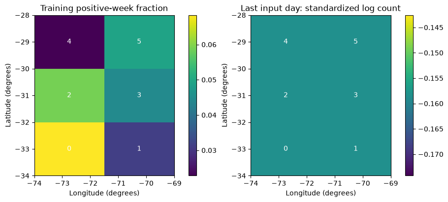
The grid has three latitude bands and two longitude bands. Row zero is the southern band; column zero is the western band. Cell IDs increase west to east within a row, then south to north. These rectangles provide a simple teaching representation; they are not inferred tectonic regions and do not have equal physical areas.
For each forecast origin, X_train contains 30 maps × 3 rows × 2 columns × 3 channels. Its target is a 3 × 2 binary map. Several cells may contain an event in the same target week, or all may be zero.
We keep these dimensions visible throughout model fitting. Flattened six-cell arrays are used only to display tables later.
Code block 7 · Run the matching prepared-notebook cell in order. For self-study, copy into a new Colab code cell.
N_CELLS = N_ROWS * N_COLS

X_train = X_grid[train_mask].astype("float32")
X_val = X_grid[val_mask].astype("float32")
y_train = y_grid[train_mask].astype("float32")
y_val = y_grid[val_mask].astype("float32")
validation_origins = origins[val_mask]

print("Training histories:", X_train.shape)
print("Training targets:  ", y_train.shape)
print("Validation histories:", X_val.shape)
print("Validation targets:  ", y_val.shape)

lat_centres = (LAT_EDGES[:-1] + LAT_EDGES[1:]) / 2
lon_centres = (LON_EDGES[:-1] + LON_EDGES[1:]) / 2
cell_table = pd.DataFrame({
    "cell": np.arange(N_CELLS),
    "latitude": np.repeat(lat_centres, N_COLS),
    "longitude": np.tile(lon_centres, N_ROWS),
    "training_positive_weeks": y_train.sum(axis=0).ravel().astype(int),
    "training_prevalence": y_train.mean(axis=0).ravel(),
})
display(cell_table)
Verified local output · single seed — expand to compare
Training histories: (834, 30, 3, 2, 3)
Training targets:   (834, 3, 2)
Validation histories: (208, 30, 3, 2, 3)
Validation targets:   (208, 3, 2)
| cell | latitude | longitude | training_positive_weeks | training_prevalence | |
|---|---|---|---|---|---|
| 0 | 0 | -33.0 | -72.75 | 57 | 0.068345 |
| 1 | 1 | -33.0 | -70.25 | 26 | 0.031175 |
| 2 | 2 | -31.0 | -72.75 | 49 | 0.058753 |
| 3 | 3 | -31.0 | -70.25 | 37 | 0.044365 |
| 4 | 4 | -29.0 | -72.75 | 19 | 0.022782 |
| 5 | 5 | -29.0 | -70.25 | 41 | 0.049161 |
The first map below shows the fraction of training weeks with a positive outcome in each cell. The second shows the last input day for the first training origin. Its colours represent a standardized input channel, not raw counts. Small numbers of positive weeks limit how much a model can learn for a cell.
Discuss: What geographic information would disappear if these six daily values were reduced to one regional count?
Code block 8 · Run the matching prepared-notebook cell in order. For self-study, copy into a new Colab code cell.
training_prevalence = y_train.mean(axis=0)
example_day = X_train[0, -1, :, :, 0]

fig, axes = plt.subplots(1, 2, figsize=(9, 4), constrained_layout=True)
fields = [training_prevalence, example_day]
titles = ["Training positive-week fraction", "Last input day: standardized log count"]
for ax, field, title in zip(axes, fields, titles):
    image = ax.pcolormesh(LON_EDGES, LAT_EDGES, field, cmap="viridis", shading="flat")
    for cell in range(N_CELLS):
        row, column = divmod(cell, N_COLS)
        ax.text(lon_centres[column], lat_centres[row], str(cell),
                ha="center", va="center", color="white")
    ax.set(title=title, xlabel="Longitude (degrees)", ylabel="Latitude (degrees)")
    fig.colorbar(image, ax=ax)
plt.show()
Verified local output · single seed — expand to compare
A reference forecast before neural networks
Predict each cell’s training prevalence for every validation week. This reference captures persistent differences between cells without adapting to the preceding 30 days. It uses no validation labels to fit its probabilities.
Brier score is the mean squared error of the probabilities. Log loss gives a larger penalty to confident incorrect probabilities. Smaller values are better for both. Here we average over all validation weeks and all six cells; these are marginal probability scores, not a joint spatial likelihood.
Code block 9 · Run the matching prepared-notebook cell in order. For self-study, copy into a new Colab code cell.
p_baseline = np.broadcast_to(training_prevalence, y_val.shape).copy()

brier_baseline = np.mean((p_baseline - y_val) ** 2)
p_safe = np.clip(p_baseline.astype(float), 1e-7, 1 - 1e-7)
logloss_baseline = -np.mean(y_val * np.log(p_safe) + (1 - y_val) * np.log1p(-p_safe))

print("Baseline Brier score:", round(float(brier_baseline), 6))
print("Baseline log loss:   ", round(float(logloss_baseline), 6))
Verified local output · single seed — expand to compare
Baseline Brier score: 0.045091
Baseline log loss:    0.191246
Model 1: apply the same CNN to every day, then use an LSTM
TimeDistributed(Conv2D) applies the same spatial filters to each of the 30 daily maps. It does not fit 30 different CNNs. Flatten turns each day’s feature map into a vector while retaining fixed spatial positions. The LSTM then reads the sequence of 30 vectors.
The intermediate objects show each step directly:
| Object | Shape for one history | Meaning |
|---|---|---|
daily_maps |
(30, 3, 2, 3) |
Observed map sequence |
spatial_features |
(30, 3, 2, 8) |
Eight learned spatial channels per day |
daily_vectors |
(30, 48) |
One vector per day |
temporal_state |
(16,) |
Summary of the map history |
probability_map |
(3, 2) |
Six weekly occurrence probabilities |
We use six sigmoid outputs because events can occur in several cells. Their probabilities need not sum to one. The sigmoid outputs do not assume that the underlying seismic processes are independent.
Code block 10 · Run the matching prepared-notebook cell in order. For self-study, copy into a new Colab code cell.
keras.backend.clear_session()
keras.utils.set_random_seed(SEED)

daily_maps = keras.Input(shape=X_train.shape[1:], name="daily_maps")
spatial_features = keras.layers.TimeDistributed(
    keras.layers.Conv2D(8, kernel_size=3, padding="same", activation="relu"),
    name="shared_daily_convolution",
)(daily_maps)
daily_vectors = keras.layers.TimeDistributed(
    keras.layers.Flatten(), name="daily_vectors",
)(spatial_features)
temporal_state = keras.layers.LSTM(16, name="temporal_memory")(daily_vectors)
cell_probabilities = keras.layers.Dense(
    N_CELLS, activation="sigmoid", name="cell_probabilities",
)(temporal_state)
probability_map = keras.layers.Reshape(
    (N_ROWS, N_COLS), name="probability_map",
)(cell_probabilities)

model_cnn2d = keras.Model(daily_maps, probability_map, name="cnn2d_lstm")
model_cnn2d.compile(
    optimizer=keras.optimizers.Adam(learning_rate=0.001),
    loss=keras.losses.BinaryCrossentropy(),
)
model_cnn2d.summary()
Verified local output · single seed — expand to compare
WARNING:tensorflow:From C:\Users\Francisco Plaza\AppData\Local\Temp\statsei14-transformer-pilot-20261007\Lib\site-packages\keras\src\backend\common\global_state.py:82: The name tf.reset_default_graph is deprecated. Please use tf.compat.v1.reset_default_graph instead.
Model: "cnn2d_lstm"
┏━━━━━━━━━━━━━━━━━━━━━━━━━━━━━━━━━┳━━━━━━━━━━━━━━━━━━━━━━━━┳━━━━━━━━━━━━━━━┓
┃ Layer (type)                    ┃ Output Shape           ┃       Param # ┃
┡━━━━━━━━━━━━━━━━━━━━━━━━━━━━━━━━━╇━━━━━━━━━━━━━━━━━━━━━━━━╇━━━━━━━━━━━━━━━┩
│ daily_maps (InputLayer)         │ (None, 30, 3, 2, 3)    │             0 │
├─────────────────────────────────┼────────────────────────┼───────────────┤
│ shared_daily_convolution        │ (None, 30, 3, 2, 8)    │           224 │
│ (TimeDistributed)               │                        │               │
├─────────────────────────────────┼────────────────────────┼───────────────┤
│ daily_vectors (TimeDistributed) │ (None, 30, 48)         │             0 │
├─────────────────────────────────┼────────────────────────┼───────────────┤
│ temporal_memory (LSTM)          │ (None, 16)             │         4,160 │
├─────────────────────────────────┼────────────────────────┼───────────────┤
│ cell_probabilities (Dense)      │ (None, 6)              │           102 │
├─────────────────────────────────┼────────────────────────┼───────────────┤
│ probability_map (Reshape)       │ (None, 3, 2)           │             0 │
└─────────────────────────────────┴────────────────────────┴───────────────┘
Total params: 4,486 (17.52 KB)
Trainable params: 4,486 (17.52 KB)
Non-trainable params: 0 (0.00 B)
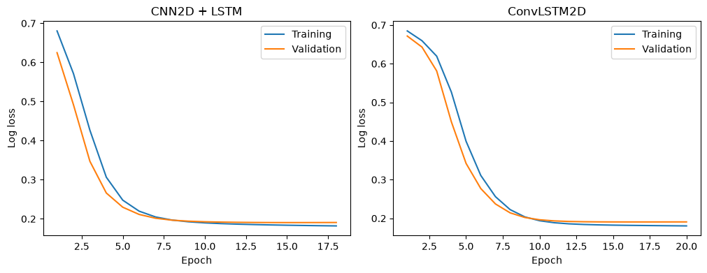
Fit this model once. Early stopping monitors validation log loss and restores the best weights after three epochs without improvement. The maximum is 20 epochs, with batches of 64 histories. The LSTM state restarts for each history.
Discuss: Which operation connects neighbouring cells, and which one connects successive days?
Code block 11 · Run the matching prepared-notebook cell in order. For self-study, copy into a new Colab code cell.
stopping_cnn2d = keras.callbacks.EarlyStopping(
    monitor="val_loss", patience=3, restore_best_weights=True,
)
start = time.perf_counter()
history_cnn2d = model_cnn2d.fit(
    X_train, y_train,
    validation_data=(X_val, y_val),
    epochs=EPOCHS, batch_size=BATCH_SIZE,
    callbacks=[stopping_cnn2d], shuffle=False, verbose=2,
)
seconds_cnn2d = time.perf_counter() - start
p_cnn2d = model_cnn2d.predict(X_val, batch_size=BATCH_SIZE, verbose=0)

brier_cnn2d = np.mean((p_cnn2d - y_val) ** 2)
p_safe = np.clip(p_cnn2d.astype(float), 1e-7, 1 - 1e-7)
logloss_cnn2d = -np.mean(y_val * np.log(p_safe) + (1 - y_val) * np.log1p(-p_safe))
print("Prediction shape:", p_cnn2d.shape)
Verified local output · single seed — expand to compare
Epoch 1/20
14/14 - 2s - 126ms/step - loss: 0.6805 - val_loss: 0.6249
Epoch 2/20
14/14 - 0s - 8ms/step - loss: 0.5713 - val_loss: 0.4917
Epoch 3/20
14/14 - 0s - 7ms/step - loss: 0.4266 - val_loss: 0.3472
Epoch 4/20
14/14 - 0s - 7ms/step - loss: 0.3064 - val_loss: 0.2661
Epoch 5/20
14/14 - 0s - 8ms/step - loss: 0.2478 - val_loss: 0.2298
Epoch 6/20
14/14 - 0s - 8ms/step - loss: 0.2196 - val_loss: 0.2113
Epoch 7/20
14/14 - 0s - 7ms/step - loss: 0.2048 - val_loss: 0.2016
Epoch 8/20
14/14 - 0s - 7ms/step - loss: 0.1969 - val_loss: 0.1966
Epoch 9/20
14/14 - 0s - 7ms/step - loss: 0.1925 - val_loss: 0.1940
Epoch 10/20
14/14 - 0s - 8ms/step - loss: 0.1897 - val_loss: 0.1926
Epoch 11/20
14/14 - 0s - 7ms/step - loss: 0.1878 - val_loss: 0.1917
Epoch 12/20
14/14 - 0s - 7ms/step - loss: 0.1865 - val_loss: 0.1911
Epoch 13/20
14/14 - 0s - 8ms/step - loss: 0.1854 - val_loss: 0.1908
Epoch 14/20
14/14 - 0s - 7ms/step - loss: 0.1845 - val_loss: 0.1906
Epoch 15/20
14/14 - 0s - 7ms/step - loss: 0.1837 - val_loss: 0.1905
Epoch 16/20
14/14 - 0s - 7ms/step - loss: 0.1831 - val_loss: 0.1905
Epoch 17/20
14/14 - 0s - 7ms/step - loss: 0.1825 - val_loss: 0.1906
Epoch 18/20
14/14 - 0s - 7ms/step - loss: 0.1820 - val_loss: 0.1907
Prediction shape: (208, 3, 2)
Model 2: maintain a spatial state with ConvLSTM2D
ConvLSTM2D uses convolutions inside its recurrent updates. Its state therefore keeps a row and column dimension while it reads the daily maps. We flatten only the final spatial state, then predict the same six targets.
The input is unchanged. This model uses four recurrent feature channels, giving a final spatial state of (3, 2, 4) and a flattened vector of length 24. Its parameter count differs from the first model: a common training protocol does not imply equal capacity or computation.
Code block 12 · Run the matching prepared-notebook cell in order. For self-study, copy into a new Colab code cell.
keras.backend.clear_session()
keras.utils.set_random_seed(SEED)

daily_maps = keras.Input(shape=X_train.shape[1:], name="daily_maps")
spatial_state = keras.layers.ConvLSTM2D(
    filters=4, kernel_size=3, padding="same", return_sequences=False,
    name="spatiotemporal_memory",
)(daily_maps)
final_vector = keras.layers.Flatten(name="final_spatial_state")(spatial_state)
cell_probabilities = keras.layers.Dense(
    N_CELLS, activation="sigmoid", name="cell_probabilities",
)(final_vector)
probability_map = keras.layers.Reshape(
    (N_ROWS, N_COLS), name="probability_map",
)(cell_probabilities)

model_convlstm = keras.Model(daily_maps, probability_map, name="convlstm")
model_convlstm.compile(
    optimizer=keras.optimizers.Adam(learning_rate=0.001),
    loss=keras.losses.BinaryCrossentropy(),
)
model_convlstm.summary()
Verified local output · single seed — expand to compare
Model: "convlstm"
┏━━━━━━━━━━━━━━━━━━━━━━━━━━━━━━━━━┳━━━━━━━━━━━━━━━━━━━━━━━━┳━━━━━━━━━━━━━━━┓
┃ Layer (type)                    ┃ Output Shape           ┃       Param # ┃
┡━━━━━━━━━━━━━━━━━━━━━━━━━━━━━━━━━╇━━━━━━━━━━━━━━━━━━━━━━━━╇━━━━━━━━━━━━━━━┩
│ daily_maps (InputLayer)         │ (None, 30, 3, 2, 3)    │             0 │
├─────────────────────────────────┼────────────────────────┼───────────────┤
│ spatiotemporal_memory           │ (None, 3, 2, 4)        │         1,024 │
│ (ConvLSTM2D)                    │                        │               │
├─────────────────────────────────┼────────────────────────┼───────────────┤
│ final_spatial_state (Flatten)   │ (None, 24)             │             0 │
├─────────────────────────────────┼────────────────────────┼───────────────┤
│ cell_probabilities (Dense)      │ (None, 6)              │           150 │
├─────────────────────────────────┼────────────────────────┼───────────────┤
│ probability_map (Reshape)       │ (None, 3, 2)           │             0 │
└─────────────────────────────────┴────────────────────────┴───────────────┘
Total params: 1,174 (4.59 KB)
Trainable params: 1,174 (4.59 KB)
Non-trainable params: 0 (0.00 B)
The fit is written out again so the model, inputs, loss and stopping rule remain visible. We use the same seed and a new early-stopping callback.
Code block 13 · Run the matching prepared-notebook cell in order. For self-study, copy into a new Colab code cell.
stopping_convlstm = keras.callbacks.EarlyStopping(
    monitor="val_loss", patience=3, restore_best_weights=True,
)
start = time.perf_counter()
history_convlstm = model_convlstm.fit(
    X_train, y_train,
    validation_data=(X_val, y_val),
    epochs=EPOCHS, batch_size=BATCH_SIZE,
    callbacks=[stopping_convlstm], shuffle=False, verbose=2,
)
seconds_convlstm = time.perf_counter() - start
p_convlstm = model_convlstm.predict(X_val, batch_size=BATCH_SIZE, verbose=0)

brier_convlstm = np.mean((p_convlstm - y_val) ** 2)
p_safe = np.clip(p_convlstm.astype(float), 1e-7, 1 - 1e-7)
logloss_convlstm = -np.mean(y_val * np.log(p_safe) + (1 - y_val) * np.log1p(-p_safe))
print("Prediction shape:", p_convlstm.shape)
Verified local output · single seed — expand to compare
Epoch 1/20
14/14 - 1s - 74ms/step - loss: 0.6849 - val_loss: 0.6717
Epoch 2/20
14/14 - 0s - 16ms/step - loss: 0.6596 - val_loss: 0.6432
Epoch 3/20
14/14 - 0s - 16ms/step - loss: 0.6196 - val_loss: 0.5814
Epoch 4/20
14/14 - 0s - 15ms/step - loss: 0.5266 - val_loss: 0.4496
Epoch 5/20
14/14 - 0s - 16ms/step - loss: 0.3994 - val_loss: 0.3421
Epoch 6/20
14/14 - 0s - 15ms/step - loss: 0.3110 - val_loss: 0.2771
Epoch 7/20
14/14 - 0s - 15ms/step - loss: 0.2560 - val_loss: 0.2372
Epoch 8/20
14/14 - 0s - 16ms/step - loss: 0.2225 - val_loss: 0.2141
Epoch 9/20
14/14 - 0s - 16ms/step - loss: 0.2037 - val_loss: 0.2022
Epoch 10/20
14/14 - 0s - 16ms/step - loss: 0.1938 - val_loss: 0.1963
Epoch 11/20
14/14 - 0s - 16ms/step - loss: 0.1886 - val_loss: 0.1933
Epoch 12/20
14/14 - 0s - 16ms/step - loss: 0.1858 - val_loss: 0.1919
Epoch 13/20
14/14 - 0s - 16ms/step - loss: 0.1841 - val_loss: 0.1912
Epoch 14/20
14/14 - 0s - 16ms/step - loss: 0.1831 - val_loss: 0.1908
Epoch 15/20
14/14 - 0s - 16ms/step - loss: 0.1824 - val_loss: 0.1907
Epoch 16/20
14/14 - 0s - 18ms/step - loss: 0.1818 - val_loss: 0.1906
Epoch 17/20
14/14 - 0s - 17ms/step - loss: 0.1815 - val_loss: 0.1906
Epoch 18/20
14/14 - 0s - 16ms/step - loss: 0.1811 - val_loss: 0.1906
Epoch 19/20
14/14 - 0s - 16ms/step - loss: 0.1808 - val_loss: 0.1907
Epoch 20/20
14/14 - 0s - 16ms/step - loss: 0.1804 - val_loss: 0.1907
Prediction shape:
(208, 3, 2)
Compare with the reference forecast
These are single-run validation scores for seed 7. The rows are shown in teaching order. They are not estimates of a universal ranking of model families. Runtime describes this execution environment.
Discuss: Does either spatial model improve both scores over cell prevalence? How much improvement is visible relative to the added parameters? A lower score from a more complex model is not guaranteed.
Code block 14 · Run the matching prepared-notebook cell in order. For self-study, copy into a new Colab code cell.
comparison = pd.DataFrame({
    "model": ["Cell prevalence", "CNN2D + LSTM", "ConvLSTM2D"],
    "seed": [None, SEED, SEED],
    "brier": [brier_baseline, brier_cnn2d, brier_convlstm],
    "log_loss": [logloss_baseline, logloss_cnn2d, logloss_convlstm],
    "network_parameters": [0, model_cnn2d.count_params(), model_convlstm.count_params()],
    "epochs": [0, len(history_cnn2d.history["loss"]), len(history_convlstm.history["loss"])],
    "fit_seconds": [0, seconds_cnn2d, seconds_convlstm],
})
display(comparison.round(6))

fig, axes = plt.subplots(1, 2, figsize=(10, 3.8), constrained_layout=True)
for ax, name, history in zip(
    axes, ["CNN2D + LSTM", "ConvLSTM2D"], [history_cnn2d, history_convlstm],
):
    epochs = np.arange(1, len(history.history["loss"]) + 1)
    ax.plot(epochs, history.history["loss"], label="Training")
    ax.plot(epochs, history.history["val_loss"], label="Validation")
    ax.set(title=name, xlabel="Epoch", ylabel="Log loss")
    ax.legend()
plt.show()
Verified local output · single seed — expand to compare
| model | seed | brier | log_loss | network_parameters | epochs | fit_seconds | |
|---|---|---|---|---|---|---|---|
| 0 | Cell prevalence | NaN | 0.045091 | 0.191246 | 0 | 0 | 0.000000 |
| 1 | CNN2D + LSTM | 7.0 | 0.045069 | 0.190481 | 4486 | 18 | 3.583696 |
| 2 | ConvLSTM2D | 7.0 | 0.044992 | 0.190606 | 1174 | 20 | 5.312600 |
Check the six cells separately
An average over all cells can hide a poor result in one location. The table below retains every cell and shows its validation support. Counts refer to positive forecast weeks, not independent earthquakes.
The spatial scores cannot be ranked against the regional tutorial’s scores: the outcomes and their positive fractions differ.
Code block 15 · Run the matching prepared-notebook cell in order. For self-study, copy into a new Colab code cell.
cell_scores = cell_table[["cell", "latitude", "longitude"]].copy()
cell_scores["validation_positive_weeks"] = y_val.sum(axis=0).ravel().astype(int)
cell_scores["observed_fraction"] = y_val.mean(axis=0).ravel()
cell_scores["brier_prevalence"] = np.mean((p_baseline - y_val) ** 2, axis=0).ravel()
cell_scores["brier_cnn2d_lstm"] = np.mean((p_cnn2d - y_val) ** 2, axis=0).ravel()
cell_scores["brier_convlstm"] = np.mean((p_convlstm - y_val) ** 2, axis=0).ravel()
display(cell_scores.round(5))
Verified local output · single seed — expand to compare
| cell | latitude | longitude | validation_positive_weeks | observed_fraction | brier_prevalence | brier_cnn2d_lstm | brier_convlstm | |
|---|---|---|---|---|---|---|---|---|
| 0 | 0 | -33.0 | -72.75 | 10 | 0.04808 | 0.04618 | 0.04588 | 0.04511 |
| 1 | 1 | -33.0 | -70.25 | 6 | 0.02885 | 0.02802 | 0.02832 | 0.02818 |
| 2 | 2 | -31.0 | -72.75 | 14 | 0.06731 | 0.06285 | 0.06336 | 0.06381 |
| 3 | 3 | -31.0 | -70.25 | 13 | 0.06250 | 0.05892 | 0.05853 | 0.05830 |
| 4 | 4 | -29.0 | -72.75 | 9 | 0.04327 | 0.04182 | 0.04157 | 0.04162 |
| 5 | 5 | -29.0 | -70.25 | 7 | 0.03365 | 0.03276 | 0.03275 | 0.03294 |
Interpret a probability map
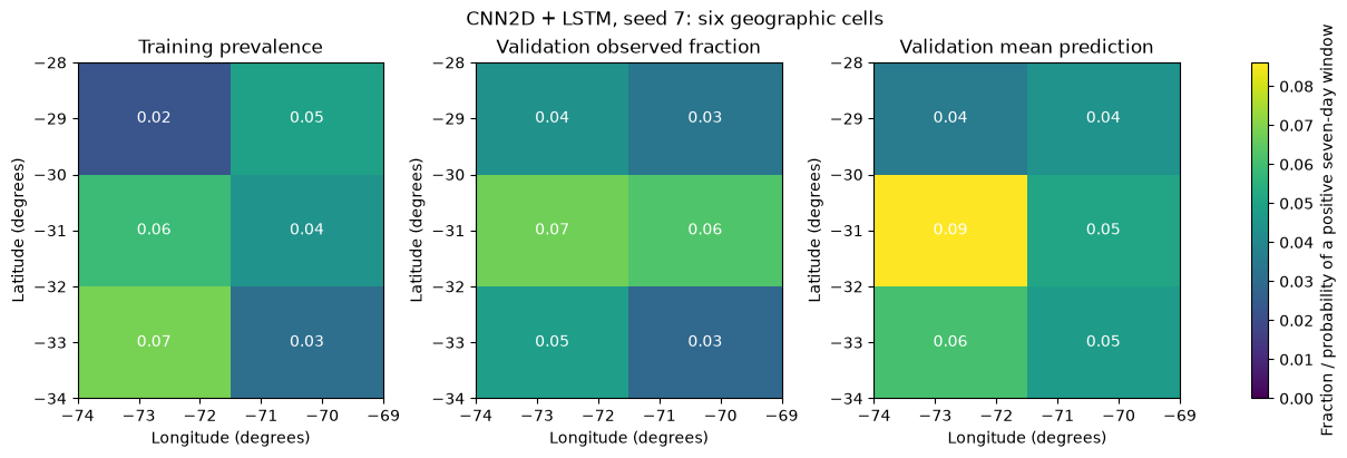
For illustration we use CNN2D + LSTM, seed 7, chosen before comparing scores. The third map averages its probabilities across validation weeks. It is not the forecast for a single week. Agreement between spatial averages alone does not establish calibration.
Each colour describes catalogue occurrence within a cell and a seven-day horizon. It does not describe the intensity of shaking.
Code block 16 · Run the matching prepared-notebook cell in order. For self-study, copy into a new Colab code cell.
observed_map = y_val.mean(axis=0)
predicted_map = p_cnn2d.mean(axis=0)
map_fields = [training_prevalence, observed_map, predicted_map]
map_titles = ["Training prevalence", "Validation observed fraction", "Validation mean prediction"]
colour_limit = max(float(field.max()) for field in map_fields)

fig, axes = plt.subplots(1, 3, figsize=(12, 4), constrained_layout=True)
for ax, field, title in zip(axes, map_fields, map_titles):
    image = ax.pcolormesh(
        LON_EDGES, LAT_EDGES, field, vmin=0, vmax=max(colour_limit, 0.01),
        cmap="viridis", shading="flat",
    )
    for cell in range(N_CELLS):
        row, column = divmod(cell, N_COLS)
        ax.text(lon_centres[column], lat_centres[row], f"{field[row, column]:.2f}",
                ha="center", va="center", color="white")
    ax.set(title=title, xlabel="Longitude (degrees)", ylabel="Latitude (degrees)")
fig.colorbar(image, ax=axes, label="Fraction / probability of a positive seven-day window")
fig.suptitle(f"CNN2D + LSTM, seed {SEED}: six geographic cells")
plt.show()
Verified local output · single seed — expand to compare
Optional: calibration of the same individual run
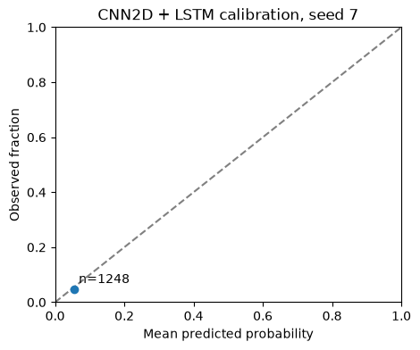
Group the CNN2D + LSTM probabilities into five fixed bins. Within each bin, compare the mean prediction with the observed fraction. The same seed-7 probabilities are used here and in the score table; no ensemble is formed.
Inspect the number of origin–cell pairs and positives in each bin. A point based on few positive outcomes provides limited evidence. Spatial cells and forecast weeks can be dependent, so the plot is descriptive. Pooling can also conceal differences among cells.
Code block 17 · Run the matching prepared-notebook cell in order. For self-study, copy into a new Colab code cell.
bin_edges = np.linspace(0, 1, 6)
probability_bin = np.minimum(
    np.searchsorted(bin_edges, p_cnn2d.ravel(), side="right") - 1, 4,
)
calibration_data = pd.DataFrame({
    "bin": probability_bin,
    "probability": p_cnn2d.ravel(),
    "observed": y_val.ravel(),
})
calibration = calibration_data.groupby("bin").agg(
    origin_cell_pairs=("observed", "size"),
    positives=("observed", "sum"),
    mean_probability=("probability", "mean"),
    observed_fraction=("observed", "mean"),
)
display(calibration)

fig, ax = plt.subplots(figsize=(5, 4))
ax.plot([0, 1], [0, 1], "--", color="grey")
ax.plot(calibration.mean_probability, calibration.observed_fraction, "o")
for row in calibration.itertuples():
    ax.annotate(f"n={row.origin_cell_pairs}", (row.mean_probability, row.observed_fraction),
                xytext=(4, 5), textcoords="offset points")
ax.set(xlim=(0, 1), ylim=(0, 1), xlabel="Mean predicted probability",
       ylabel="Observed fraction", title=f"CNN2D + LSTM calibration, seed {SEED}")
plt.show()
Verified local output · single seed — expand to compare
| origin_cell_pairs | positives | mean_probability | observed_fraction | |
|---|---|---|---|---|
| bin | ||||
| 0 | 1248 | 59.0 | 0.054096 | 0.047276 |
Save this individual run
Export validation scores and predictions with their origin, cell where relevant, and seed. The protocol table records the fixed split and checksums. These files describe one run; the three-seed reference results remain separate. Rerunning with another seed writes into the same folder, so copy that folder before another run.
Code block 18 · Run the matching prepared-notebook cell in order. For self-study, copy into a new Colab code cell.
output_dir = Path("outputs_maps")
output_dir.mkdir(exist_ok=True)
predictions = pd.DataFrame({
    "origin": np.repeat(validation_origins.astype(str), N_CELLS),
    "cell": np.tile(np.arange(N_CELLS), len(y_val)),
    "observed": y_val.astype(int).ravel(),
    "baseline_probability": p_baseline.ravel(),
    "cnn2d_lstm_probability": p_cnn2d.ravel(),
    "convlstm_probability": p_convlstm.ravel(),
    "seed": SEED,
})
comparison.to_csv(output_dir / "validation_metrics.csv", index=False)
cell_scores.to_csv(output_dir / "validation_metrics_by_cell.csv", index=False)
predictions.to_csv(output_dir / "validation_predictions.csv", index=False)
pd.DataFrame(history_cnn2d.history).to_csv(output_dir / "cnn2d_training_history.csv", index_label="epoch_zero_based")
pd.DataFrame(history_convlstm.history).to_csv(output_dir / "convlstm_training_history.csv", index_label="epoch_zero_based")
print("Tables saved to:", output_dir.resolve())

protocol = pd.DataFrame([{
    "seed": SEED, "lookback_days": LOOKBACK, "horizon_days": HORIZON,
    "train_start": "2001-01-01", "train_end_exclusive": "2017-01-01",
    "validation_start": "2017-01-01", "validation_end_exclusive": "2021-01-01",
    "training_examples": int(train_mask.sum()), "validation_examples": int(val_mask.sum()),
    "maximum_epochs": EPOCHS, "batch_size": BATCH_SIZE, "early_stopping_patience": 3,
    "pack_sha256": PACK_SHA256, "catalogue_sha256": CATALOGUE_SHA256,
    "tensorflow_version": tf.__version__, "keras_version": keras.__version__,
    "historical_as_of_verified": False, "colab_execution_verified": False,
}])
protocol.to_csv(output_dir / "protocol.csv", index=False)
Verified local output · single seed — expand to compare
Tables saved to: H:\Otros ordenadores\Mi PC\1_Proyectos\2026 - Statsei 14 -\statsei14-deep-learning\qa\linear-integration-2026-10-07\executions\maps-72a90c96ba\outputs_maps
What to take forward
- Explain which operation acts on space and which acts on time in each model.
- Compare with cell prevalence before discussing which neural model is better.
- Keep the cell-level objective separate from the regional objective.
- Continue with the graph tutorial using the same six cells, inputs and targets. Inputs, targets and partitions stay fixed; the architecture changes how spatial and temporal information is shared.
Repeating the two fits with seeds 17 and 27 is a follow-up exercise, not a hidden part of this notebook. Report every specified run. Variation across seeds describes optimization variability rather than uncertainty from a new earthquake catalogue. The three-seed reference comparison retains those repeated runs and the detailed export workflow. An untouched period would be needed to assess performance independently of development decisions.
Sources and continuation
- Complete map tutorial and three-seed results
- Graph tutorial on the same cells
- Keras TimeDistributed
- Keras Conv2D
- Keras LSTM
- Keras ConvLSTM2D
The Keras references explain the layers’ mechanics; they do not establish the forecasting performance of this catalogue experiment.